Article

Using Visual Ozone Damage Scores and Spectroscopy to Quantify Soybean Responses to Background Ozone

1
Department of Earth and Atmospheric Sciences, Saint Louis University, St. Louis, MO 63108, USA
2
Geospatial Institute, Saint Louis University, 3694 West Pine Mall, St. Louis, MO 63108, USA
3
Department of Mathematics and Natural Sciences, Harris-Stowe State University, St. Louis, MO 63103, USA
*
Author to whom correspondence should be addressed.
Remote Sens. 2020, 12(1), 93; https://doi.org/10.3390/rs12010093
Submission received: 1 November 2019 / Revised: 23 December 2019 / Accepted: 23 December 2019 / Published: 26 December 2019
(This article belongs to the Section Remote Sensing in Agriculture and Vegetation)

Abstract

:
Remotely-sensed identification of ozone stress in crops can allow for selection of ozone resistant genotypes, improving yields. This is critical as population, food demand, and background tropospheric ozone are projected to increase over the next several decades. Visual scores of common ozone damage have been used to identify ozone-stress in bio-indicator plants. This paper evaluates the use of a visual scoring metric of ozone damage applied to soybeans. The scoring of the leaves is then combined with hyperspectral data to identify spectral indices specific to ozone damage. Two genotypes of soybean, Dwight and Pana, that have shown different sensitivities to ozone, were grown and visually scored for ozone-specific damage on multiple dates throughout the growing season. Leaf reflectance, foliar biophysical properties, and yield data were collected. Additionally, ozone bio-indicator plants, snap beans, and common milkweed, were investigated with visual scores and hyperspectral leaf data for comparison. The normalized difference spectral index (NDSI) was used to identify the significant bands in the visible (VIS), near infrared (NIR), and shortwave infrared (SWIR) that best correlated with visual damage score when used in the index. Results were then compared to multiple well-established indices. Indices were also evaluated for correlation with seed and pod weight. The ozone damage scoring metric for soybeans evaluated in August had a coefficient of determination of 0.60 with end-of-season pod weight and a Pearson correlation coefficient greater than 0.6 for photosynthetic rate, stomatal conductance, and transpiration. NDSI [R558, R563] correlated best with visual scores of ozone damage in soybeans when evaluating data from all observation dates. These wavelengths were similar to those identified as most sensitive to visual damage in August when used in NDSI (560 nm, 563 nm). NDSI [R560, R563] in August had the highest coefficient of determination for individual pod weight (R2 = 0.64) and seed weight (R2 = 0.54) when compared against 21 well-established indices used for identification of pigment or photosynthetic stress in plants. When evaluating use of spectral bands in NDSI, longer wavelengths in SWIR were identified as more sensitive to ozone visual damage. Trends in the bands and biophysical properties of the soybeans combined with evaluation of ozone data indicate likely timing of significant ozone damage as after late-July for this season. This work has implications for better spectral detection of ozone stress in crops and could help with efforts to identify ozone tolerant varieties to increase future yield.

Graphical Abstract

1. Introduction

Despite regulations placed on pollutants, tropospheric ozone levels are projected to increase in polluted regions with a warming climate [1]. Concentrations are often higher in rural areas downwind of major pollution centers, often the locations of agricultural production [2,3]. High ozone concentrations during the summer months, have been shown to negatively influence crop growth and yield through impacts on leaf-level photosynthesis as well as damages to whole-canopy physiology [4]. Soybeans are among the crops that are vulnerable to tropospheric ozone concentrations, and global relative yield losses in 2008 were estimated to be between 6% and 16% [5]. Soybean yield losses on the order of 10% were estimated in the Midwest of the United States in 2005 [6,7]. Although regionally dependent, global yield losses due to ambient ozone are projected to increase, posing a threat to global food security [8].
Visual symptoms on ozone-sensitive plants have long been used to aid in pollution monitoring and to understand the effects of ozone on these various species. In the western United States, significant work has been done using pines as bioindicators of ozone damage [9]. Additionally, symptoms such as chlorotic mottling in conifer species have been used to monitor tropospheric ozone in the Pyrenees Mountains in Spain [10]. The impact of ozone on trees is covered in detail by Matyssek et al. [11]. Additional agricultural species, including tobacco plants [12] and snap beans [13] have been evaluated as bioindicator species of ozone. Results have shown significant relationship between foliar injury in tobacco plants and measures of ambient ozone, AOT40, and AOT20 [12]. In Europe, an urban air quality assessment network, the EuroBionet, uses ozone sensitive plants as indicators of air quality [14].
Identification of plant genotypes that are more tolerant to ozone and more likely to have high productivity in future climates is essential to meeting future projections for global food demand [15]. Selecting crop varieties with ozone resistance could greatly improve agricultural production [8]. Ozone-induced damage to crops is associated with decreases in photosynthesis and also leads to visible damage on the leaf, such as accelerated senescence, decreased leaf area, reduction in leaf green area [16], and cell death resulting in necrosis of plant cells [17]. Many studies have documented ozone-induced leaf injury on species that are particularly ozone sensitive [18]. These species, such as snap bean, common milkweed, and cutleaf coneflower are good bioindicators of ozone-induced injury [13,19,20]. A field guide for how to score ozone damage based on foliar systems was developed by experts in tropospheric ozone and plant physiology and is available online at https://science-edu.larc.nasa.gov/ozonegarden/pdf/Bio-guide-final-3_15_11.pdf [21]. Visual foliar damage of ozone can also be detected in soybeans [22,23].
Using visible signs of ozone damage on plants aids in optical remote sensing detection of ozone stress on plant species. Studies have shown that reflectance in the visible bands was most sensitive to ozone damage in crop species due to chlorosis symptoms, the yellowing of the leaves due to foliar loss of chlorophyll [24,25]. Hyperspectral data, in particular, can better show the increase in visible (VIS) reflectance in ozone damaged plants, specifically in the region of chlorophyll absorption (590–690 nm) and Ustin and Curtiss et al. (1990) recommended high spectral resolution (5 nm) for ozone stress detection after investigating the applicability of using various spectral resolutions to detect ozone-induced spectral variation in tree species [26]. Spectral reflectance indices have been used to evaluate ozone effects on plants including identifying changes in photochemical reflectance index (PRI) in plants exposed to elevated ozone [27,28]. PRI can be a useful index for soybean leaf assessment of ozone stress [29] because of its indication of de-epoxidation of the xanthophyll pigments, a phenomenon that has been reported to occur in biochemical analyses of plants exposed to elevated ozone [30,31]. Previous studies have also evaluated PRI and other spectral indices for several soybean genotypes at various ozone concentrations [32].
No studies, however, have used visually scored soybean leaves as indicators of specific leaves under ozone stress combined with high resolution leaf reflectance measurements to identify a normalized difference spectral index (NDSI) specific to ozone stress. In this study, we examine the potential of using visual ozone damage scores of chlorosis and necrosis, developed by experts in surface ozone and plant physiology, on two genotypes of soybeans with differing ozone sensitivity as well as two other bioindicator species, common milkweed and two genotypes of snap beans, to identify specific spectral bands sensitive to ozone damage. The bioindicator species were included for comparison purposes because the visual scoring protocol was developed for these plants that show specific symptoms when exposed to high levels of ambient ozone. In addition to identifying NDSI best correlated to the visual scores for all three species, use of high resolution spectral bands (3 and 9 nm widths) are also investigated as current and future hyperspectral satellite missions like EnMAP and HyspIRI will have 10 nm spectral resolution.
For the soybean genotypes, the newly developed NDSI as well as several existing indices are examined for correlations to seed and pod weight. Several studies have investigated the use of vegetation indices to predict crop yield for multiple species [33,34], including soybeans [35,36]. An index specific to ozone damage, such as the NDSI developed in this study, may be useful to incorporate into yield prediction as well.
The application of the visual scoring system to soybeans is evaluated by its correlation to end-of-season seed and pod weight as well as to physiological changes in leaves exposed to high ozone concentrations such as photosynthetic rate [37,38,39,40] and stomatal conductance [41,42]. Studies have shown that with increasing time that ambient ozone levels are above 40 ppb, photosynthetic rate decreases [43]; hence, comparing photosynthetic rate in ozone sensitive and ozone tolerant varieties and investigating correlations between ozone damage scores and photosynthetic rate is important to evaluate whether the leaf scores can be used to help detect remotely-sensed ozone stress on the plants. Stomatal conductance and transpiration rates have also been studied for soybeans grown in differing ozone concentrations and were reduced at higher concentrations, so they may also be helpful for evaluating the leaf scoring protocol [44,45]. Correlating visual ozone damage scores to seed and pod weight is new to this study; however, multiple studies have shown reduction in seed weight and yield that have correlated to ambient ozone levels [7,8,46,47]. In this study, we also investigate 8-h average ozone concentrations for the growing season in accordance with temporal patterns of ozone sensitive spectral bands and physiological properties of the soybean leaves to identify likely timing of ozone damage on the plants.

2. Materials and Methods

2.1. Experimental Site

An ozone garden was established in 2012 at the Saint Louis Science Center (SLSC) in St. Louis, MO, USA (38° 37′ N, 90° 16′ W). The garden is an educational and public outreach facility allowing for both observing and quantifying ozone damage to plants. Several bio-indicator plants that show pronounced visual symptoms of ozone damage are grown at this location to increase public awareness of the effects of high levels of tropospheric ozone. In 2015, 16 plants of two genotypes of soybean (Glycine max) were grown along with 12 plants of common milkweed (Asclepias syriaca), and 16 plants of two genotypes of snap beans (Phaseolus vulgaris). The soybean varieties, Dwight (O3 sensitive) and Pana (O3 tolerant), were selected for their previously shown sensitivities to ozone [48]. An ozone sensitive (S156) and tolerant (R123) variety of snap bean were also selected. The garden was planted in early May with the soybeans and snap beans in two rows each with 12-inch spacing between plants, therefore soil conditions, including soil moisture levels, were kept the same for both genotypes of the snap beans and soybeans. This allowed for the foliar visual and biophysical differences between the genotypes to be isolated to their sensitivities to ambient ozone.

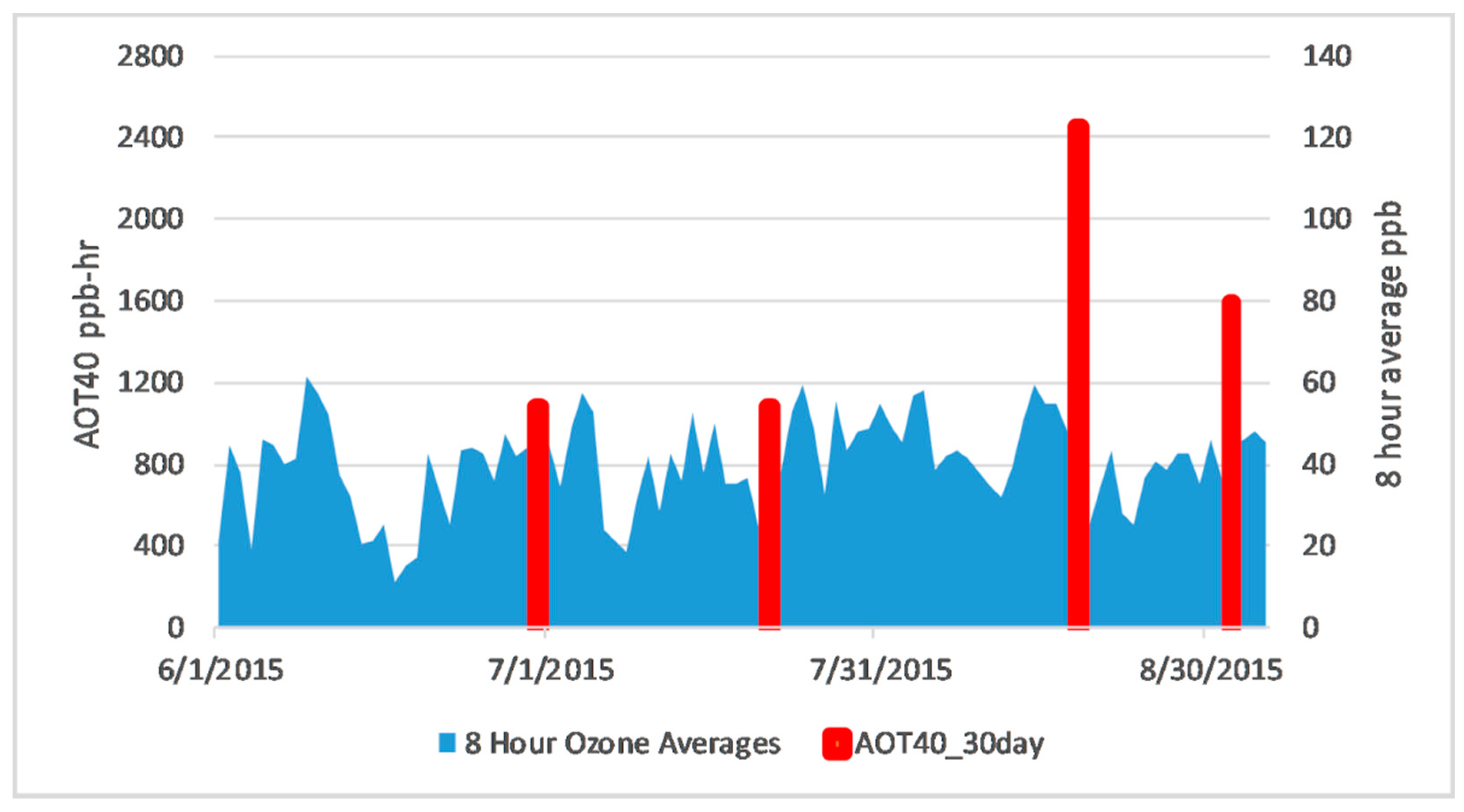
2.2. Background Ozone

An ozone monitor, (Model 106-L, 2BTechnologies, Boulder, CO, USA), providing 15-minute resolution ambient ozone concentration data, was present on-site. Measurements are available at http://go3project.com/network2/index.php/pages/ozone-data. The readings have been shown to be consistent with archived data at Missouri’s Department of Natural Resources (DNR). Data was missing for July and August and was imputed using data from nearby sites at Grant’s Farm and Southwestern Illinois College; locations also a part of the GO3 network. Linear regression was used to predict missing ozone concentrations at SLSC based on ozone concentrations and atmospheric conditions at the other two sites. Atmospheric conditions were included in the model based on correlations with ozone. The method was validated using data from 2014, which did not have gaps in the data for July and August. The mean difference between actual and imputed ozone levels for 2014 data was 2.0 ppb and fifty percent of the differences were between –1.6 ppb and 5.2 ppb. Once data was imputed from the neighboring stations, 8-h average ozone concentrations from 10:00 am–5:00 pm were then calculated along with AOT40, a measure of the ozone concentrations above 40 ppb, for 30 days prior to each observation date. Ozone concentrations of 40 ppb have been shown to be a critical threshold for ozone damage to vegetation [49,50,51]. For this study, the hours and concentration of ozone above 40 ppb increased from 1089 ppb h for the 30 days prior to 21 July to 2456 ppb h for the 30 days prior to 18 August (Figure 1).

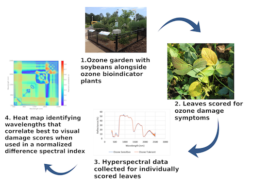
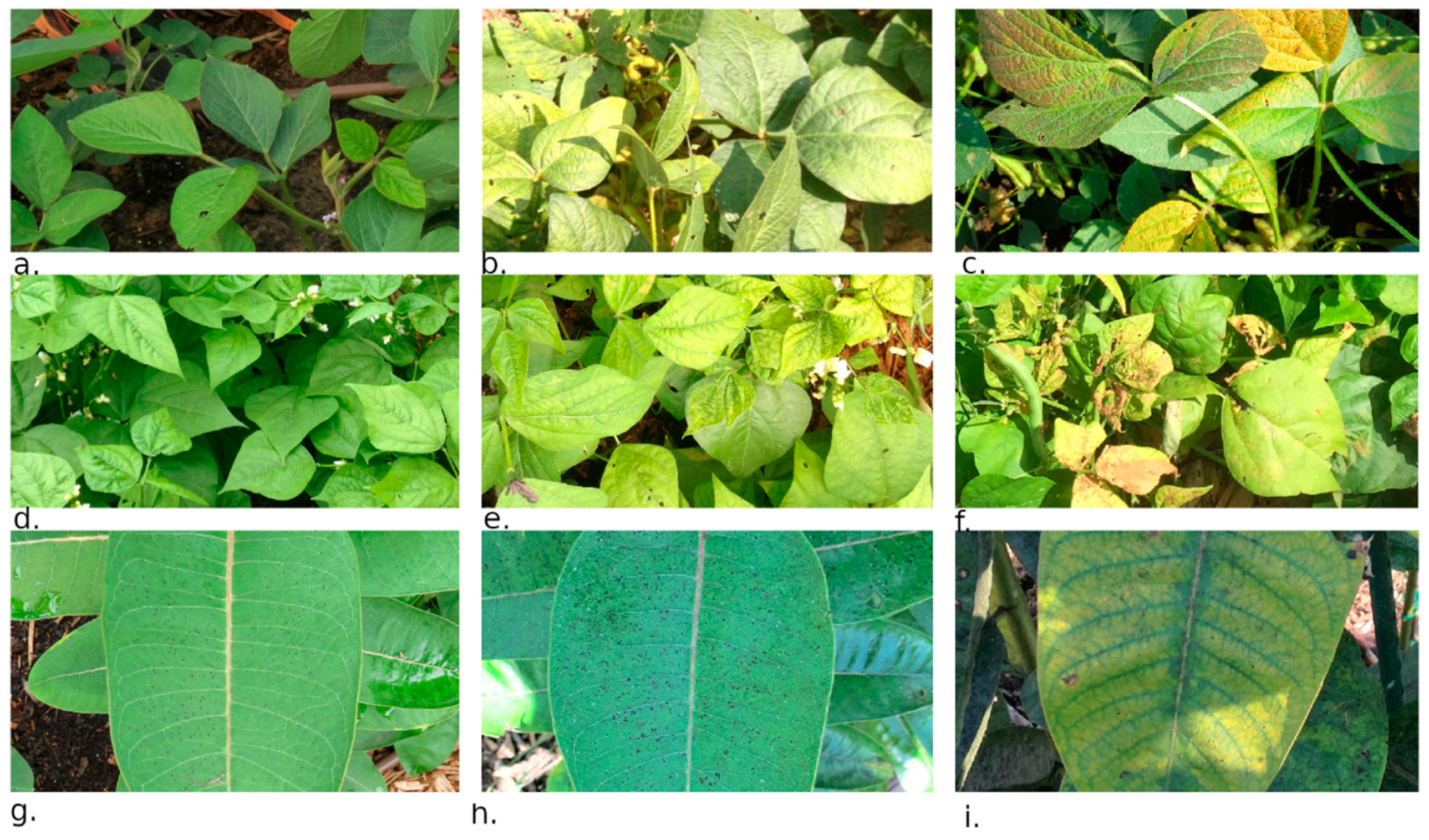
2.3. Visual Scoring of Ozone Damage

Visual damage of common foliar ozone symptoms was examined for each of the plant species throughout the growing season. Soybeans were scored on five separate days between late June and early September. Single leaves of each plant were scored for chlorosis, necrosis, and stippling, common ozone-related symptoms, and given a score for each category based on the percentage of the leaf damaged. The same individual scored all plants following guidelines from Ladd et al.’s Ozone-Induced Foliar Injury Field Guide [21]. Care was taken to identify ozone related damage, distinguished from other types of damage such as mold or insects. Stippling for soybean leaves was never more than a score of 2 and scoring was dropped after mid-July. Beginning 18 August 2015, soybean plants were given a whole plant score and a leaf representative of the score was chosen for spectral and physiological measurements. The protocol was changed and new leaves representative of the whole plant score were selected at this point because of the loss of several leaves that had been marked and were scored prior to August. Common milkweed leaves were scored in all three categories on six separate dates throughout the growing season. Snap beans were harvested in late-July and were only given visual scores on two separate dates prior to harvest. Photographs of progression of visible foliar ozone damage from each plant species are shown in Figure 2.

2.4. Leaf Spectral Data

Both soybean genotypes, snap bean genotypes, and the common milkweed plants were measured for their VIS, near infrared (NIR), and shortwave infrared (SWIR) (350–2500 nm) reflectance using a high-resolution full-range PSR+ 3500 (portable spectroradiometer, Spectral Revolution, Inc. Lawrence, MA, USA). A leaf clip with an integrated white reference and light source was used with the PSR+ 3500 to obtain high resolution leaf reflectance of a 3 mm spot on the same leaves that were scored for ozone damage for each plant species. In June and July, spectral signatures were collected for the specific leaves that were visually scored for ozone damage. For August and September, however, the plant was given a whole plant visual score and spectral signatures were collected for the leaf most representative of that score. All measurements were taken between 10:00 a.m.–12:00 p.m. during clear skies on four separate days for the soybeans and common milkweed between 30 June 2015 and 1 September 2015 and on two separate days (30 June 2015 and 21 July 2015) for the snap beans. Observation dates for each species are presented in Table 1.
Because 3 samples were taken for each plant and then averaged together, a total of 192 spectral samples from 64 different plants were collected for the soybeans, 78 spectral samples from 26 plants for the snap beans, and 117 spectral samples from 39 plants for the common milkweed.

2.5. Leaf Gas Exchange, Photosynthetic Rate, and Chlorophyll Content

Each leaf that was selected for spectral analysis was also analyzed simultaneously for gas-exchange variables and fluorescence variables, including photosynthetic rate, stomatal conductance, and transpiration using the LI-6400XT Portable Photosynthesis System installed with a pulse amplitude-modulated leaf chamber fluorometer (Li-Cor, Inc., Lincoln, NE, USA). The Dualex Scientific+TM (ForceA, France) was also used on each selected plant leaf to simultaneously obtain chlorophyll, flavonol, anthocyanin, and nitrogen balance indices. This instrument uses optical absorbance at 375 nm and transmittance at 3 wavelengths in the NIR to estimate chlorophyll, flavonol, and anthocyanin content. The Dualex Scientific+TM uses a chemical calibration to give chlorophyll values in µg/cm2, while flavonol and anthocyanin content are given in relative absorbance units. Both the LI-6400XT Portable Photosynthesis System and Dualex Scientific+TM measurements were taken simultaneously with the spectral samples in June, July, and August, however, the LI-6400XT measurements were not taken in September.

2.6. Pod and Seed Weight Data

Soybeans were hand-harvested on 2 October 2015, at the end of the growing season. Harvesting took place when the pods were dry on the plants and they were laid out to dry further at room temperature before weight measurements were taken. After pods were dried, pod weight for each plant of both genotypes was measured. Pods were then manually removed and seed weight for each plant was measured. Because pod and seed development takes place at different growing stages, this study investigates the relationship with each variable and visual damage scores individually [52].

2.7. Statistical Analysis Using NDSI Spectral Correlation Mapping

In order to identify spectral wavelengths that could best indicate ozone damage to the plants, the NDSI was used (Equation (1)). The NDSI is defined as:
N D S I ( i , j ) = R i R j R i + R j ,
where R is the reflectance value and subscripts are wavelengths in nm. Reflectance data from the PSR+ 3500 were interpolated to produce reflectance values for all wavelengths between 350 and 2500 nm. All possible combinations of available wavelengths (i and j) were used for NDSI calculations for each plant species and genotype and linear relationships between visual scoring of chlorosis and necrosis and NDSIs were examined. Heat maps of the absolute value of the Pearson correlation coefficient (r) between visual score and NDSI were generated using data collected throughout the growing season as well as for data collected on individual days. The heat maps were produced using python packages. Correlation arrays were created using NumPy [53] and plotted with Matplotlib [54]. The trends in generated indices across the growing season were then compared to trends in photosynthetic rate and stomatal conductance for both soybean genotypes. Additionally, correlations between the newly generated indices and seed weight data were then compared to previously published indices from relevant literature.
Reflectance values of the single wavelengths interpolated from the PSR+ 3500 measurements were averaged together for 3 and 9 nm bandwidths to produce new values representing the decreased spectral resolution. The average reflectance values for these bands were then used in NDSI to produce correlations between the visual scores and NDSI. This was done to consider application of this technique with lower spectral resolution tools.

3. Results

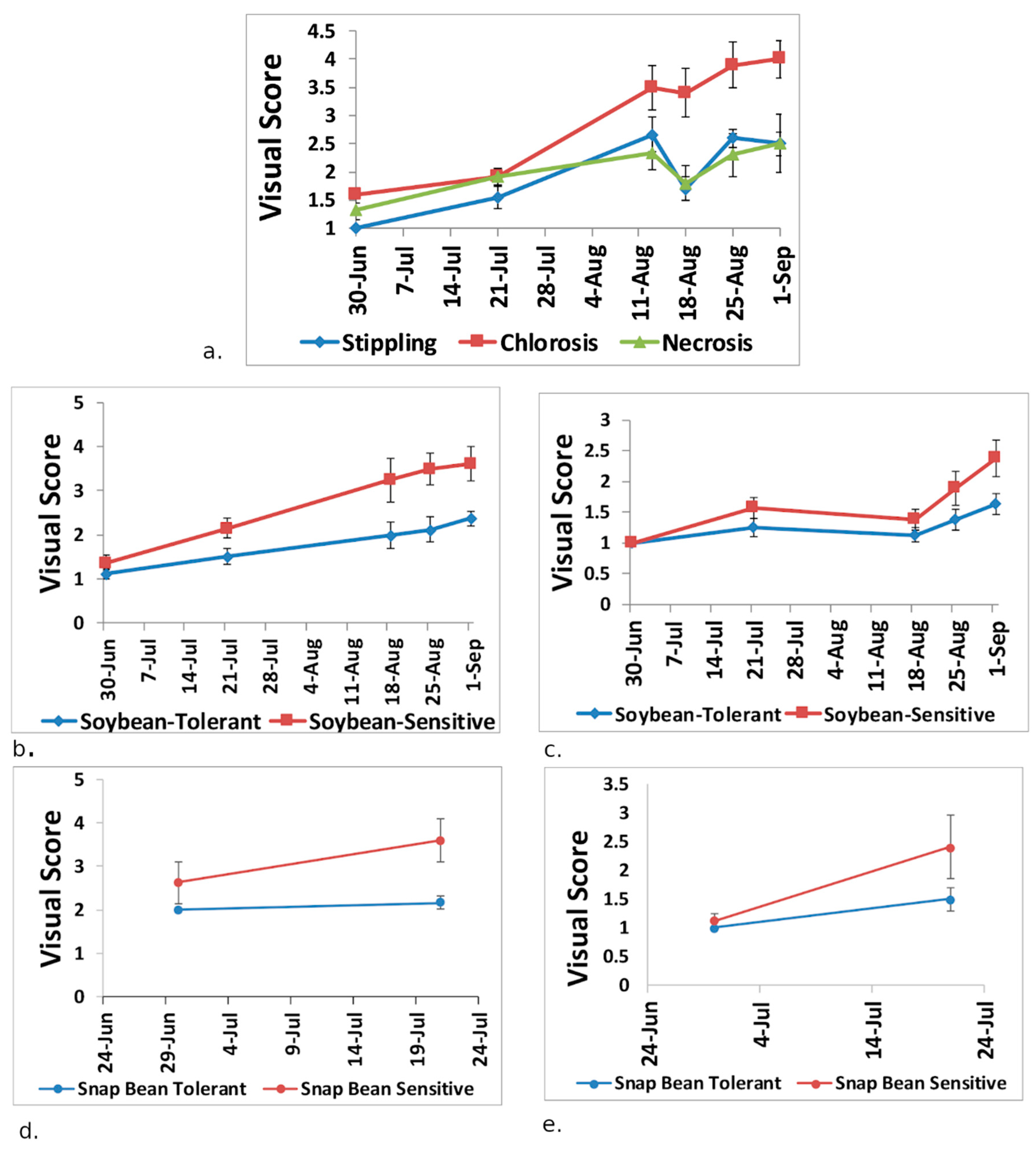
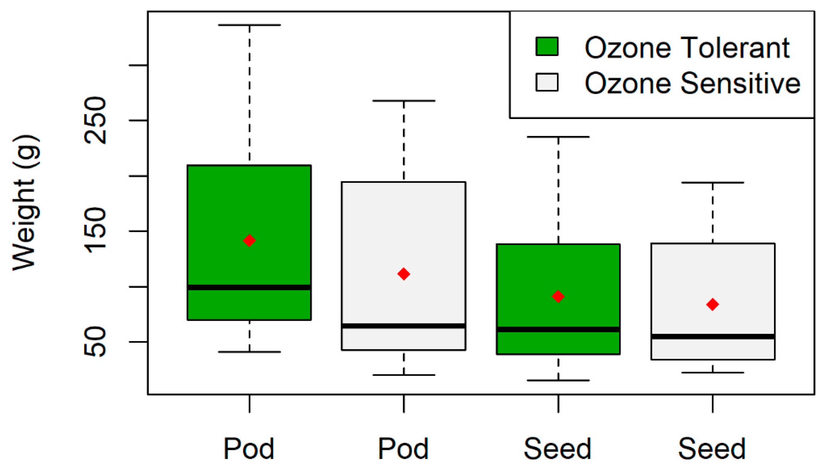
3.1. Plant Visual Scores and Seed/Pod Weight

Figure 3 shows the average visual scores for each plant species and genotype on each date. The percentage of plant damage that corresponds to each score is also shown. There is a decrease in visual necrosis score for soybeans between July and August because plant scoring was changed from a specific leaf to the whole plant beginning on 18 August 2015. For milkweed, the previously scored leaf was lost prior to 18 August 2015, so a new leaf was chosen on that date. The ozone sensitive varieties of each genotype had a greater chlorosis and necrosis score for both soybeans and snap beans and separation between the average scores for each genotype increased over time. On 21 July 2018, all soybean plants sampled had a score of 3 or lower, but by 18 August 2015, scores ranged between a 1 and a 5 for the ozone-sensitive genotype of soybean and between a 1 and a 3 for the ozone-tolerant genotype.
Seed and pod weight (g) for both soybean genotypes are shown in Figure 4. The ozone-tolerant genotype, Pana, had a greater pod and seed weight at the end of the growing season, although differences were not found to be statistically significant.
The coefficient of determination between pod weight (g) and visual score was the highest for data collected on 18 August 2015, during the plants’ reproductive growth stages. The coefficient of determination between pod weight (g) or seed weight (g) and chlorosis score was 0.60 and 0.52, respectively, in August and dropped to 0.37 and 0.28, respectively, in September. Chlorosis is more strongly correlated than necrosis with seed and pod weight. Results are shown in Table 2.

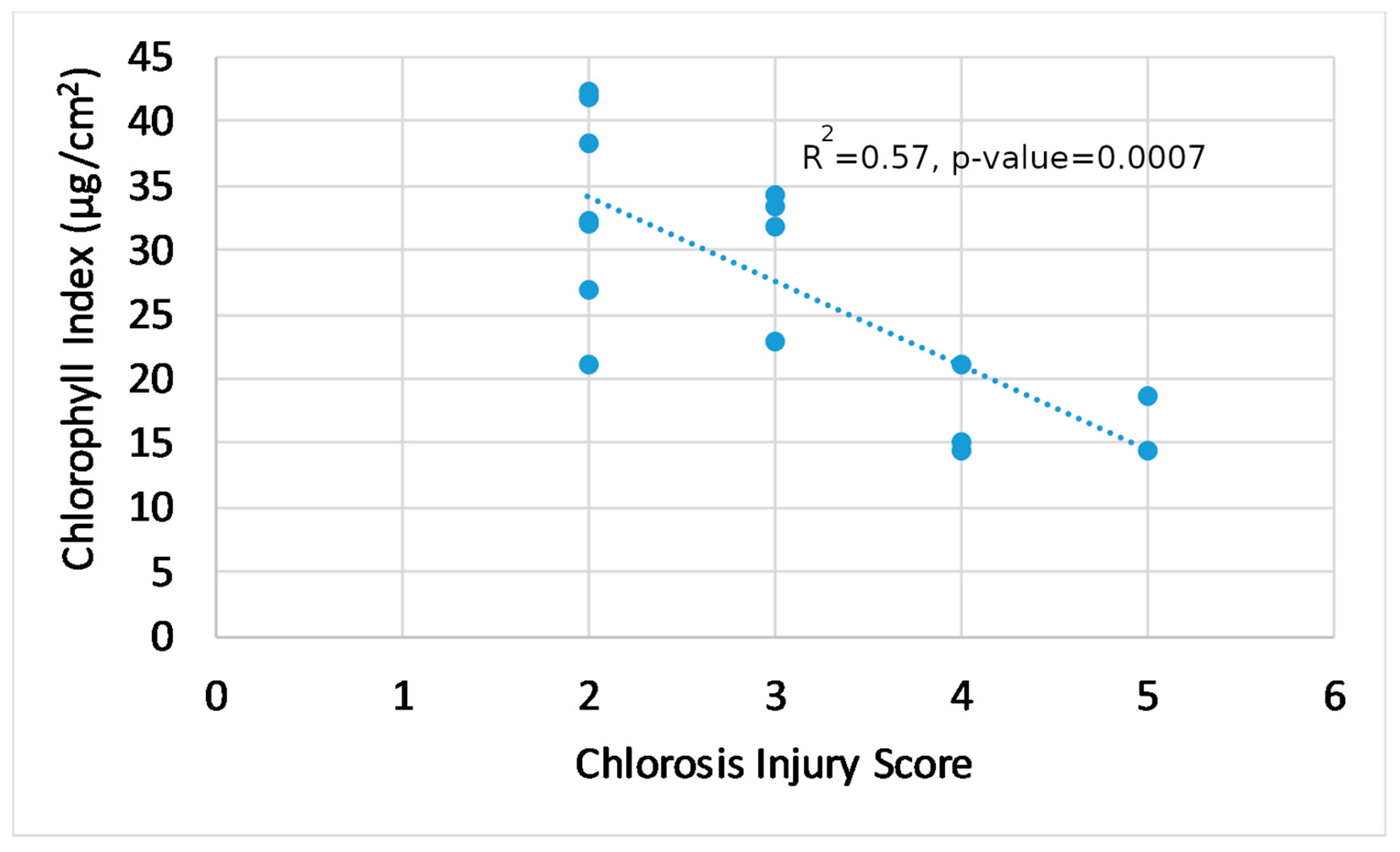
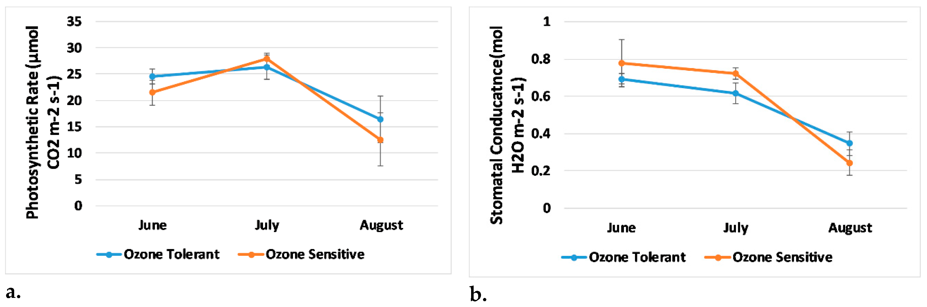
3.2. Plant Physiology and Visual Damage

When evaluating the relationship between Dualex-indicated chlorophyll index and chlorosis injury score on the last date for data collected in the growing season, the coefficient of determination between the two was determined to be 0.57. Results are shown in Figure 5. More variability is seen when damage score is lower presumably because much of the leaf is undamaged, so depending on where the measurement takes place on the leaf, chlorophyll index will vary.
Chlorosis visual score, particularly in August, also correlated well with photosynthetic rate, transpiration, and stomatal conductance (Table 3). Analysis of correlations between visual damage score and physiological variables on a particular date allows for a better comparison between the two variables than when analyzing the correlation between the variables across the entire growing season. In August, correlations between chlorosis visual score and all physiological variables were significant. Although correlations were weaker when examined across the entire growing season, correlations were still significant.

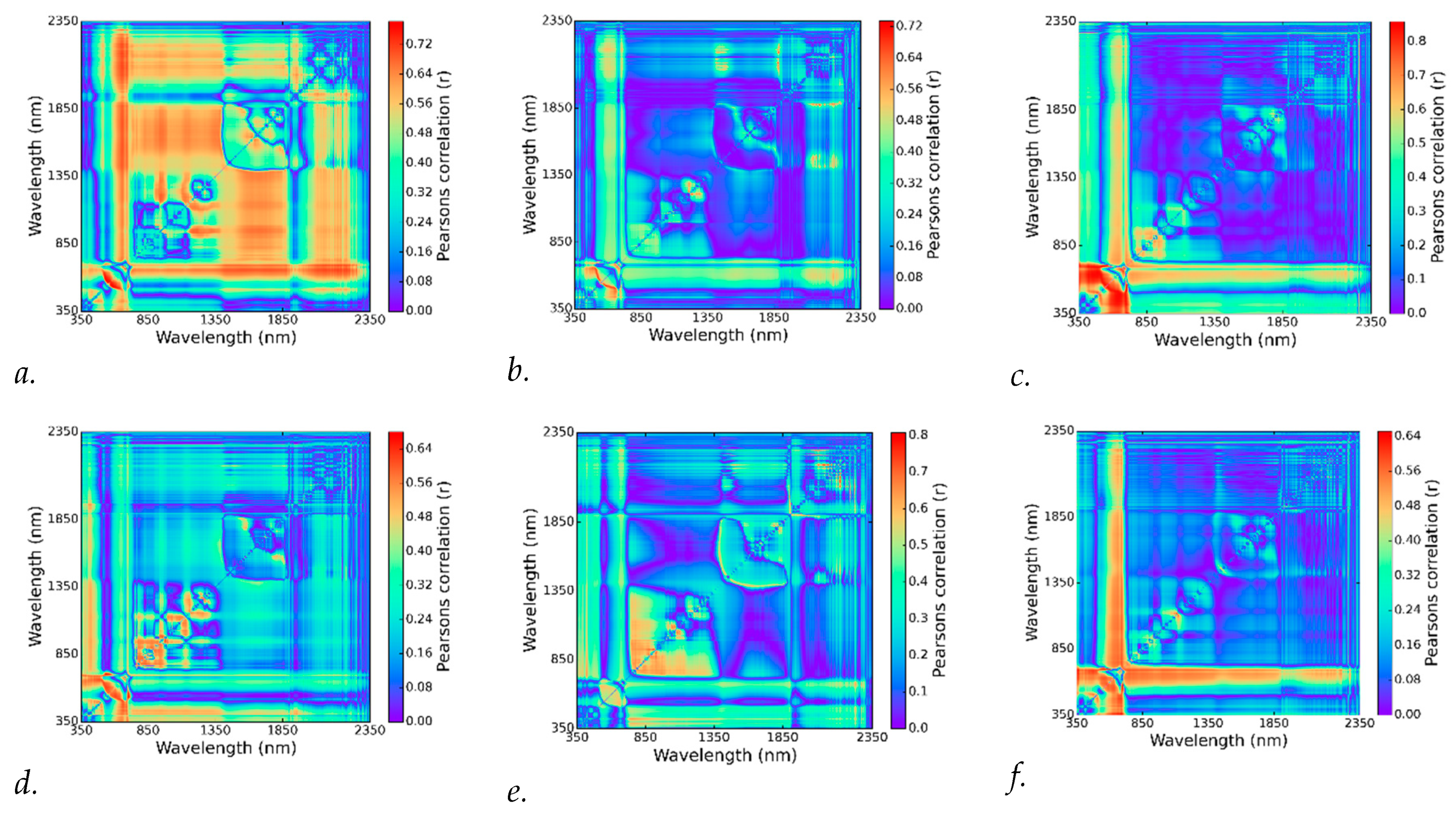
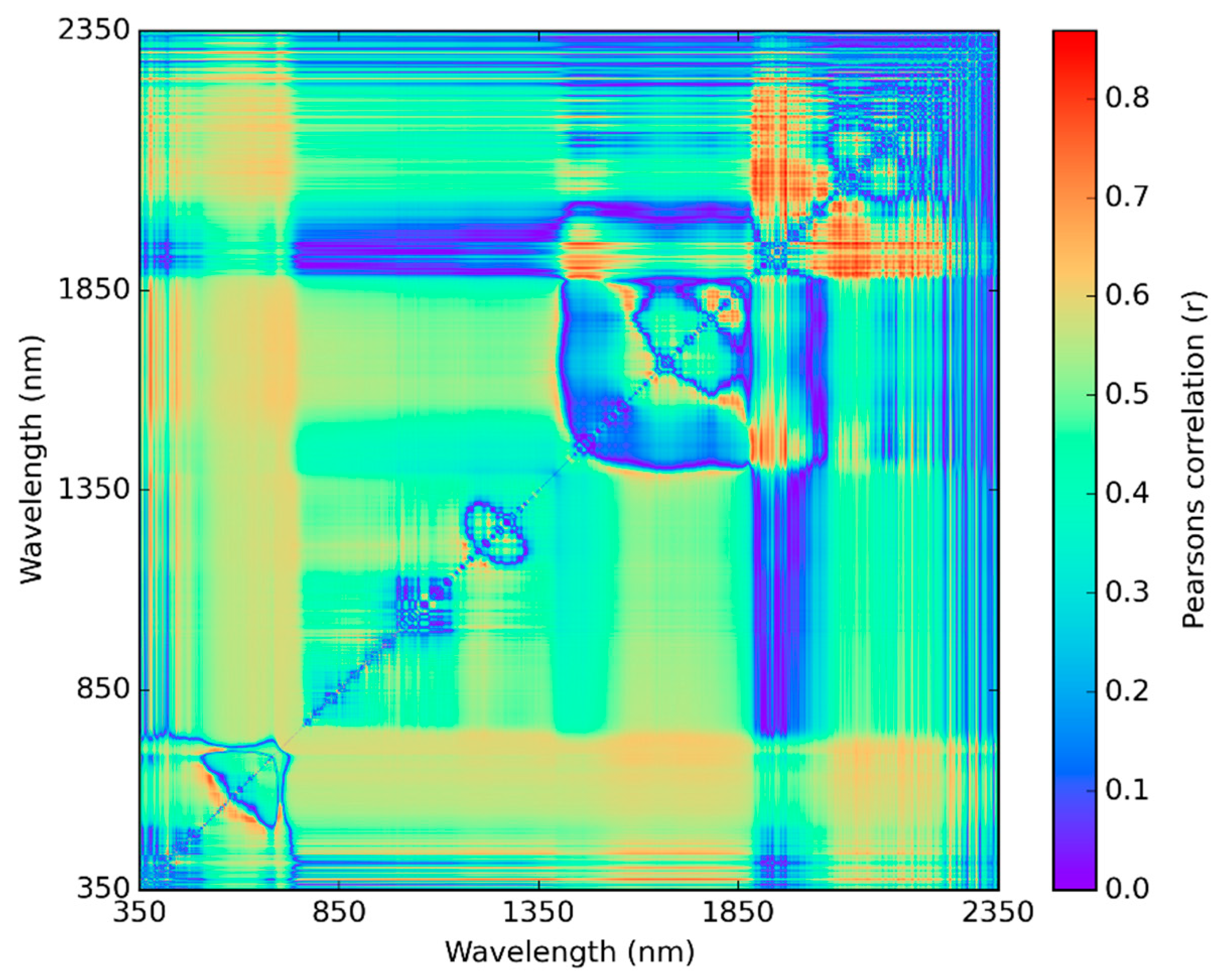
3.3. Best Spectral Regions for NDSI Correlated with Visual Scores

Determination of the best wavelengths to use for NDSI was done using all samples collected throughout the growing season, and for individual months. NDSI using single wavelengths in the mid-500 nm range had the strongest correlations with chlorosis damage score (Figure 6). For soybeans, 558 nm and 563 nm were identified as the wavelengths with the strongest correlation to chlorosis visual score across all observation dates (late June through early September) (Table 4). The top wavelengths identified when only considering samples from mid-August, when visual scores ranged from 1–5, were 560 and 563 nm, similar to the most sensitive wavelengths when considering all observation dates (Table 4) (Figure 7).
Soybeans and common milkweed showed similar wavelengths for best use in NDSI, with higher coefficients of determination between NDSI and chlorosis visual scores than for necrosis visual scores. Magnitudes of the coefficient of determination were greatest for common milkweed among the species investigated and magnitudes increased for soybeans and milkweed when investigating data from the later growing season months. However, the coefficient of determination was lower for NDSI and chlorosis scores for the snap beans. Single wavelengths in the SWIR were identified as best for use in NDSI for snap beans as opposed to the single wavelengths in the visible, mid-500 nm range for soybeans and common milkweed.
For the 3 and 9 nm resolution bands, wavelengths in the mid to upper 500 nm range were identified as the best bands correlating to chlorosis visual score, however, when considering only spectral samples collected on individual days in August and September, longer wavelengths in the SWIR were identified as having the strongest correlation (Table 4). For both soybeans and snap beans, 2140–2180 nm and 2350–2380 nm were identified as areas that correlated well with both chlorosis and necrosis visual damage scores when used in NDSI. Additionally, wavelengths around 1900 nm were successful for use in NDSI when lower resolution bands were considered for soybeans and snap beans.
Correlations using NDSI and necrosis visual score were lower than when using chlorosis visual score for both milkweed and soybeans, presumably because damage scores were much lower for necrosis, so spots of dead tissue on the leaf were more isolated. However, wavelengths in the mid-900 nm range and 660–700 nm range, when used in NDSI, had the best correlations to necrosis visual score for both soybeans and snap beans (Table 4).

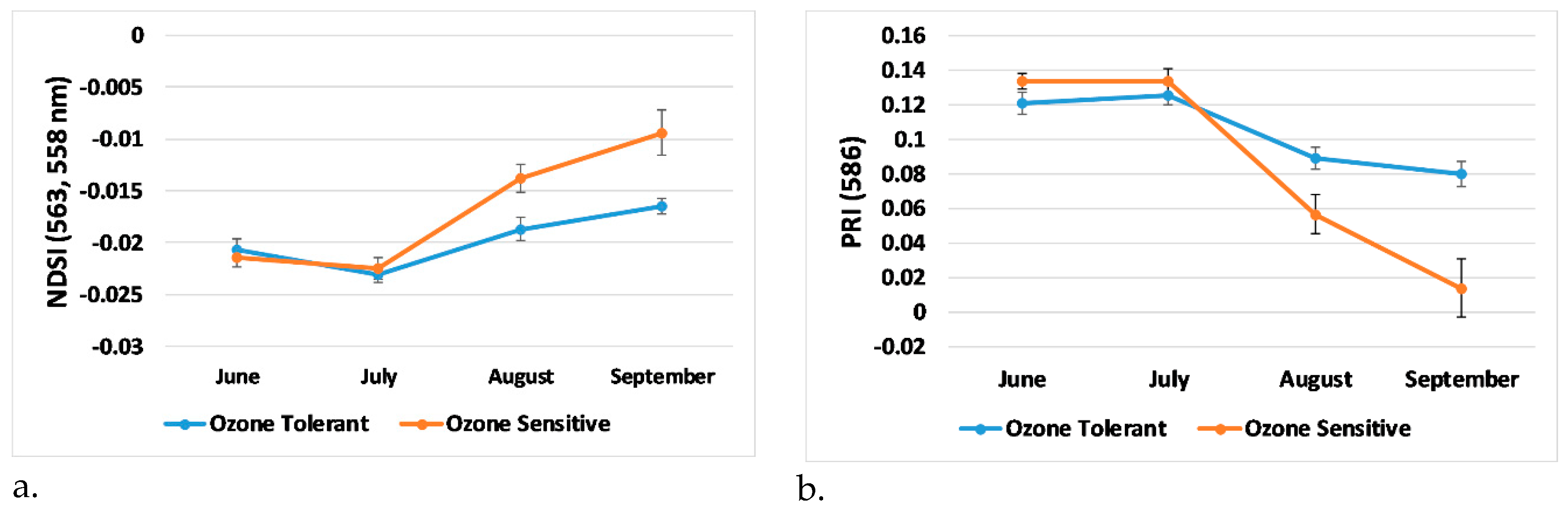
3.4. Trends in Generated Indices, Visual Score, and Plant Physiology

Trends in bands sensitive to visual score indicate a separation between the ozone sensitive and ozone tolerant genotypes of soybean after 28 July 2015 (Figure 8). Several well-established indices from relevant literature were examined for correlation with chlorosis and necrosis visual score. When using spectral samples across all dates, the photosynthetic reflective index (PRI), using 586 nm as a reference wavelength [55], correlated best with chlorosis visual scores with a coefficient of determination of 0.56. Evaluation of the trends in this band, reveled separation between the two genotypes of soybean also after 28 July 2015. Average photosynthetic rate for ozone tolerant and sensitive soybeans also switched between July and August for which genotype had a higher rate. In July, the ozone-sensitive variety had a higher average photosynthetic rate, however, the average photosynthetic rate for soybean tolerant plants was higher by 18 August 2015 (Figure 9). Additionally, evaluation of trends in stomatal conductance revealed a switch between genotypes after late July. By 18 August 2015, stomatal conductance was higher for the ozone-tolerant variety of soybean (Figure 9). However, mean differences between genotypes for both stomatal conductance and photosynthetic rate were not statistically significant in both July and August, so while there appears to be trends that support the increase of ozone damage in August, this cannot be confidently concluded with this dataset.

3.5. Comparison of Generated Indices with Existing Indices for Seed/Pod Weight Correlation

Relevant indices from the literature were also evaluated for their correlation to chlorosis visual score in August as well as to pod and seed weight (g). August was selected for examination because visual score showed the highest correlation to seed and pod weight on that date. Results are summarized in Table 5. NDSI in this study had higher coefficients of determination for chlorosis visual score, pod weight, and seed weight than other indices (Table 5). Modified triangular vegetation index (MTVI) in August had the next highest coefficient of determination for visual score in August as well as for pod and seed weight (g). MTVI has been shown to be a good predictor of green leaf area index (LAI) [56].

4. Discussion

A new metric for scoring soybean damage, based on techniques used for bio-indicator plants was developed. Average visual scores of ozone damage increased throughout the growing season for each type of plant, with the ozone sensitive variety of soybean and snap beans showing larger percentages of foliar damage. For soybeans, the damage scores best correlated to end-of-season pod and seed weight (g) when examined in August, during the reproductive growth stages of the plant. Visual damage scores in September did not correlate as strongly to seed and pod weight possibly because ozone damage occurred in some plants after pod and seed development, so these parts of the plant were not affected as much by the later ozone damage. Higher temporal resolution of data collection would allow for a more precise plant stage when visual ozone damage could best assist with yield prediction. Chlorosis damage score had a greater coefficient of determination than necrosis score for pod and seed weight. This was likely because larger areas of the leaf showed chlorosis damage, while foliar areas of necrosis were isolated. Additionally, visual damage scores on soybeans throughout the growing season showed correlations with r < –0.5 for photosynthetic rate, stomatal conductance and transpiration, variables that have been shown to be affected by ozone uptake in plants. This correlation was even stronger r < –0.6 when samples were analyzed from only the observation date in August when all other variables besides visual score of the leaves were held constant. This, along with the strong correlation in August to end-of-season seed and pod weight, give confidence to using this foliar visual scoring method to assess ozone damage on soybean plants.
When using visual damage scores to identify an NDSI best-correlated with chlorosis damage for plants and examining data across all dates throughout the growing season, single wavelengths in the mid-500 nm range worked best for both soybeans and common milkweed with specific wavelengths determined as most sensitive to chlorosis visual score when using an NDSI differing only slightly. Because chlorosis is visually seen as yellowing of the leaves, these wavelengths in the visible green-yellow range are expected, but this study identifies specific wavelengths for use in an NDSI and it is encouraging that analysis of both soybeans and common milkweed showed similar results. Although the best wavelengths identified for use in NDSI were similar for soybeans and common milkweed, the coefficient of determination was higher between NDSI and chlorosis damage scores for the common milkweed. This is possibly because it is a bioindicator plant and has a strong damage response to ambient ozone.
It is encouraging that similar wavelengths were identified as best for use in NDSI for soybeans when evaluating both the whole growing season and specific days in August and September. Evaluation of a specific day allows for only visual score to be different between the plants as all other variables are held constant. For snap beans, however, the coefficient of determination for NDSI and visual scoring was much lower than for the other two species. This is possibly because spectral observations only took place for two days for the snap beans and only in June and July, as opposed to the other plants that were observed through early September. Snap beans have a shorter growing season, so they reached senescence in July. This, along with the lower ozone levels in June and July possibly contributed to the lower coefficients of determination. Interestingly, the wavelengths identified as best for the snap beans for chlorosis, were similar to the lower resolution bands for the soybeans in August and September, closer to when the soybeans were at a similar growing stage to the snap beans in June and July. This is because the snap beans mature more quickly and were ready for harvest by late July.
Wavelengths in the VIS-red and NIR for use in NDSI were identified as most sensitive to necrosis damage for the plants investigated. Necrosis damage is reddish-brown in color and affects the foliar structure because of the dead tissue, so it is not surprising that wavelengths in these areas of the spectrum were identified as best for use in NDSI. When examining data from specific dates in August and September when more plants had larger areas of damage, longer wavelengths correlated best when lower-resolution (3 and 9 nm) bands were averaged for use in NDSI. Evaluation of lower resolution bands may be significant as satellite based remote sensing data have lower spectral resolution than the PSR+ 3500 (e.g., EnMap and HyspIRI) and these data may not be able to accurately distinguish between reflectivity from the specific identified wavelengths that are so close together (558, 563 nm). The average reflectance values from the 3 and 9 nm bandwidths that correlated well with visual score when used in an NDSI include the mid-2100 nm and mid-2300 nm ranges, and bands in the range of 1850–1950 nm. A previous study has also identified a wavelength in the mid-2300 nm range, specifically 2371 nm, as sensitive to ozone damage on soybeans [67]. SWIR reflectance has been shown to be related to lignin and cellulose content in plants, which becomes more apparent as liquid water content in the leaf decreases [73]. Studies have shown that ozone induces the biosynthesis of lignin, possibly a defense response against ozone [74]. Soybean leaves treated with ozone in field and greenhouse experiments have shown increased levels of acid-insoluble lignin although the methods used to indicate lignin content showed variable results [75]. Additionally, ozone exposure to poplar leaves led to a modification of cell wall composition that resulted in a higher lignin content [76].
The newly developed NDSI that correlated best to visual scores of ozone damage in August also correlated best to end-of-season pod and seed weight (g) when compared against multiple relevant indices found in the literature. Because all other conditions were held constant at the garden and plants were scored by an expert at identifying ozone damage, differences in visual score for plants were likely due to ozone. The developed index may be useful in identifying ozone damaged-plants and helping to predict end-of-season yield for ozone sensitive crops. PRI with 586 nm used as a reference band, also had a strong correlation to visual ozone damage. This index has been used in the past to evaluate ozone damage on plants [15,16,17,18,19,20], so it encouraging that it correlated well with visual ozone damage in this study.
Trends in averages of the spectral indices identified as best correlators with ozone damage scores showed separation between the two soybean genotypes after late-July. This matches the surface ozone observations at this location as 8-h average ozone concentrations increased in August. Evaluations of this specific band may indicate when ozone levels have begun to impact biophysical properties of the plant and help identify more specific ozone thresholds for soybeans.
Future work will include testing this methodology across multiple growing seasons and increasing sample size along with temporal resolution. Additionally, investigation of remotely-sensed indices tied to ozone visual damage scores can be examined using canopy spectral data as opposed to leaf spectral data to allow for extension of this research to airborne remote sensing tools.

5. Conclusions

This paper evaluated the use of foliar visual scores of chlorosis and necrosis at classifying soybean ozone damage as well as identifying spectral wavelengths and bands for use in a NDSI that correlates well to the visual damage. These spectral areas may be indicative of ozone damage on plants. Major conclusions were as follows:
(1)
A visual scoring system developed for bio-indicator plants was applied to soybeans to investigate the crop’s ozone damage. Correlations between foliar damage scores and physiological plant properties along with end-of-season seed and pod weight indicate this method as having potential for an ozone damage metric in soybeans.
(2)
NDSI [R563, R558] was identified as having the strongest correlation with soybean ozone damage chlorosis visual scores. Similar wavelengths were identified for common milkweed (NDSI [R558, R554]) and when data was evaluated for only the month of August (NDSI [R563, R560]) when there was a large range in chlorosis visual scores. The newly identified NDSI most sensitive to visible scores in August also had the highest correlation with soybean seed and pod weight when compared to multiple relevant indices well-established in the literature.
(3)
When evaluating the spectral bands with 3 and 9 nm bandwidth for use in an NDSI, longer wavelengths in the SWIR correlated best to chlorosis visual scores for soybeans in August and September. These bands may also indicate ozone sensitivity in soybeans due to ozone-induced changes in foliar lignin content.
(4)
Trends in newly developed NDSI showed separation between the ozone tolerant and sensitive genotypes after the July observation date. This agreed with ozone 8-h average observations along with analysis of time spent above 40 ppb for thirty days prior to each observation date, indicating that ozone had a greater effect on the soybean plants after July.

Author Contributions

Conceptualization, N.G., V.S. and J.F.; Data curation, V.S., M.M. (Matthew Maimaitiyiming), J.F. and K.B.; Formal analysis, N.G., A.P., A.B. and A.D.; Funding acquisition, V.S., J.F. and J.B.; Investigation, M.M. (Matthew Maimaitiyiming) and K.B.; Methodology, N.G. and V.S.; Project administration, V.S. and J.B.; Resources, M.M. (Maitiniyazi Maimaitijiang); Software, M.M. (Maitiniyazi Maimaitijiang); Writing–original draft, N.G.; Writing–review & editing, V.S., M.M. (Matthew Maimaitiyiming) and J.F. All authors have read and agreed to the published version of the manuscript.

Funding

This research was supported in part by NASA (NNH09ZDA001N, NNX13AB23A, NNX15AK03H), National Science Foundation (IIA-1355406 and IIA-1430427), and the Department of Education MSEIP Capacity Competitiveness Enhancement Model (CCEM) grant (P120A160064).

Acknowledgments

We gratefully acknowledge fieldwork data collection contributions from Guzhaliayi Sataer and Bethany Marshall from Saint Louis University, and Arianna Bozzolo from the University of Missouri.

Conflicts of Interest

The authors declare no conflict of interest.

References

  1. Kirtman, B.; Power, S.; Adedoyin, A.; Boer, G.; Bojariu, R.; Camilloni, I.; Doblas-Reyes, F.; Fiore, A.; Kimoto, M.; Meehl, G. Near-Term Climate Change: Projections and Predictability; Cambridge University Press: Cambridge, UK; New York, NY, USA, 2013. [Google Scholar]
  2. Fowler, D.; Amann, M.; Anderson, F.; Ashmore, M.; Cox, P.; Depledge, M.; Derwent, D.; Grennfelt, P.; Hewitt, N.; Hov, O. Ground-Level Ozone in the 21st Century: Future Trends, Impacts and Policy Implications; Royal Society Science Policy Report; Royal Society Science: London, UK, 2008; Volume 15. [Google Scholar]
  3. Xu, J.; Ma, J.; Zhang, X.; Xu, X.; Xu, X.; Lin, W.; Wang, Y.; Meng, W.; Ma, Z. Measurements of ozone and its precursors in Beijing during summertime: Impact of urban plumes on ozone pollution in downwind rural areas. Atmos. Chem. Phys. 2011, 11, 12241–12252. [Google Scholar] [CrossRef] [Green Version]
  4. Emberson, L.D.; Pleijel, H.; Ainsworth, E.A.; Van den Berg, M.; Ren, W.; Osborne, S.; Mills, G.; Pandey, D.; Dentener, F.; Büker, P. Ozone effects on crops and consideration in crop models. Eur. J. Agron. 2018, 100, 19–34. [Google Scholar] [CrossRef]
  5. Van Dingenen, R.; Dentener, F.J.; Raes, F.; Krol, M.C.; Emberson, L.; Cofala, J. The global impact of ozone on agricultural crop yields under current and future air quality legislation. Atmos. Environ. 2009, 43, 604–618. [Google Scholar] [CrossRef]
  6. Backlund, P.; Janetos, A.; Schimel, D. The Effects of Climate Change on Agriculture, Land Resources, Water Resources, and Biodiversity in the United States; Synthesis and Assessment Product 4.3; US Environmental Protection Agency, Climate Change Science Program: Washington, DC, USA, 2008; 240p. [Google Scholar]
  7. Fishman, J.; Creilson, J.K.; Parker, P.A.; Ainsworth, E.A.; Vining, G.G.; Szarka, J.; Booker, F.L.; Xu, X. An investigation of widespread ozone damage to the soybean crop in the upper Midwest determined from ground-based and satellite measurements. Atmos. Environ. 2010, 44, 2248–2256. [Google Scholar] [CrossRef]
  8. Avnery, S.; Mauzerall, D.L.; Liu, J.; Horowitz, L.W. Global crop yield reductions due to surface ozone exposure: 2. Year 2030 potential crop production losses and economic damage under two scenarios of O3 pollution. Atmos. Environ. 2011, 45, 2297–2309. [Google Scholar] [CrossRef]
  9. Miller, P.R.; Stolte, K.W.; Duriscoe, D.M.; Pronos, J. Evaluating Ozone Air Pollution Effects on Pines in the Western United States; Gen. Tech. Rep. PSW-GTR-155; Pacific Southwest Research Station, Forest Service, US Department of Agriculture: Albany, CA, USA, 1996; Volume 155, 79p. [Google Scholar]
  10. Kefauver, S.C.; Penuelas, J.; Ribas, A.; Díaz-de-Quijano, M.; Ustin, S. Using Pinus uncinata to monitor tropospheric ozone in the Pyrenees. Ecol. Indic. 2014, 36, 262–271. [Google Scholar] [CrossRef]
  11. Matyssek, R.; Sandermann, H. Impact of ozone on trees: An ecophysiological perspective. In Progress in Botany; Springer: Berlin/Heidelberg, Germany, 2003; pp. 349–404. [Google Scholar]
  12. Klumpp, A.; Ansel, W.; Klumpp, G.; Vergne, P.; Sifakis, N.; Sanz, M.J.; Rasmussen, S.; Ro-Poulsen, H.; Ribas, A.; Penuelas, J. Ozone pollution and ozone biomonitoring in European cities Part II. Ozone-induced plant injury and its relationship with descriptors of ozone pollution. Atmos. Environ. 2006, 40, 7437–7448. [Google Scholar] [CrossRef]
  13. Burkey, K.O.; Miller, J.E.; Fiscus, E.L. Assessment of ambient ozone effects on vegetation using snap bean as a bioindicator species. J. Environ. Qual. 2005, 34, 1081–1086. [Google Scholar] [CrossRef]
  14. Klumpp, A.; Ansel, W.; Klumpp, G.; Belluzzo, N.; Calatayud, V.; Chaplin, N.; Garrec, J.; Gutsche, H.; Hayes, M.; Hentze, H. EuroBionet: A pan-European biomonitoring network for urban air quality assessment. Environ. Sci. Pollut. Res. 2002, 9, 199–203. [Google Scholar] [CrossRef]
  15. Mills, G.; Sharps, K.; Simpson, D.; Pleijel, H.; Broberg, M.; Uddling, J.; Jaramillo, F.; Davies, W.J.; Dentener, F.; Van den Berg, M. Ozone pollution will compromise efforts to increase global wheat production. Glob. Chang. Biol. 2018, 24, 3560–3574. [Google Scholar] [CrossRef]
  16. Heagle, A.; Miller, J.; Pursley, W. Influence of ozone stress on soybean response to carbon dioxide enrichment: III. Yield and seed quality. Crop Sci. 1998, 38, 128–134. [Google Scholar] [CrossRef]
  17. Sandermann, H., Jr. Ozone and plant health. Annu. Rev. Phytopathol. 1996, 34, 347–366. [Google Scholar] [CrossRef] [PubMed]
  18. Mills, G.; Hayes, F.; Simpson, D.; Emberson, L.; Norris, D.; Harmens, H.; Büker, P. Evidence of widespread effects of ozone on crops and (semi-) natural vegetation in Europe (1990–2006) in relation to AOT40-and flux-based risk maps. Glob. Chang. Biol. 2011, 17, 592–613. [Google Scholar] [CrossRef] [Green Version]
  19. Chappelka, A.; Neufeld, H.; Davison, A.; Somers, G.; Renfro, J. Ozone injury on cutleaf coneflower (Rudbeckia laciniata) and crown-beard (Verbesina occidentalis) in Great Smoky Mountains National Park. Environ. Pollut. 2003, 125, 53–59. [Google Scholar] [CrossRef]
  20. Duchelle, S.; Skelly, J. The response of Asclepias syriaca to oxidant air pollution in the Shenandoah National Park of Virginia. Plant Dis. 1981, 65, 661–663. [Google Scholar] [CrossRef]
  21. Ladd, I.; Skelly, J.; Pippin, M.; Fishman, J. Ozone Induced Foliar Injury Field Guide; NASA Langley Research Center: Hampton, VA, USA, 2011. [Google Scholar]
  22. Keen, N.T.; Taylor, O. Ozone injury in soybeans: Isoflavonoid accumulation is related to necrosis. Plant Physiol. 1975, 55, 731–733. [Google Scholar] [CrossRef] [Green Version]
  23. Heagle, A.S.; Miller, J.E.; Rawlings, J.O.; Vozzo, S.F. Effect of growth stage on soybean response to chronic ozone exposure. J. Environ. Qual. 1991, 20, 562–570. [Google Scholar] [CrossRef]
  24. Cure, W.; Nusser, S.; Heagle, A. Canopy Reflectance of Soybean as Affected by Chronic Doses of Ozone in Open-Top Field Chambers; North Carolina State Univ.: Raleigh, NC, USA, 1988. [Google Scholar]
  25. Williams, J.; Ashenden, T. Differences in the spectral characteristics of white clover exposed to gaseous pollutants and acid mist. New Phytol. 1992, 120, 69–75. [Google Scholar] [CrossRef]
  26. Ustin, S.L.; Curtiss, B. Spectral characteristics of ozone-treated conifers. Environ. Exp. Bot. 1990, 30, 293–308. [Google Scholar] [CrossRef]
  27. Gamon, J.; Penuelas, J.; Field, C. A narrow-waveband spectral index that tracks diurnal changes in photosynthetic efficiency. Remote Sens. Environ. 1992, 41, 35–44. [Google Scholar] [CrossRef]
  28. Gamon, J.; Serrano, L.; Surfus, J. The photochemical reflectance index: An optical indicator of photosynthetic radiation use efficiency across species, functional types, and nutrient levels. Oecologia 1997, 112, 492–501. [Google Scholar] [CrossRef] [PubMed]
  29. Campbell, P.; Middleton, E.; McMurtrey, J.; Chappelle, E. Assessment of vegetation stress using reflectance or fluorescence measurements. J. Environ. Qual. 2007, 36, 832–845. [Google Scholar] [CrossRef] [PubMed]
  30. Castagna, A.; Nali, C.; Ciompi, S.; Lorenzini, G.; Soldatini, G.; Ranieri, A. Ozone exposure affects photosynthesis of pumpkin (Cucurbita pepo) plants. New Phytol. 2001, 152, 223–229. [Google Scholar] [CrossRef]
  31. Ranieri, A.; Giuntini, D.; Ferraro, F.; Nali, C.; Baldan, B.; Lorenzini, G.; Soldatini, G.F. Chronic ozone fumigation induces alterations in thylakoid functionality and composition in two poplar clones. Plant Physiol. Biochem. 2001, 39, 999–1008. [Google Scholar] [CrossRef]
  32. Ainsworth, E.A.; Serbin, S.P.; Skoneczka, J.A.; Townsend, P.A. Using leaf optical properties to detect ozone effects on foliar biochemistry. Photosynth. Res. 2014, 119, 65–76. [Google Scholar] [CrossRef] [PubMed]
  33. Aparicio, N.; Villegas, D.; Casadesus, J.; Araus, J.L.; Royo, C. Spectral vegetation indices as nondestructive tools for determining durum wheat yield. Agron. J. 2000, 92, 83–91. [Google Scholar] [CrossRef]
  34. Panda, S.S.; Ames, D.P.; Panigrahi, S. Application of vegetation indices for agricultural crop yield prediction using neural network techniques. Remote Sens. 2010, 2, 673–696. [Google Scholar] [CrossRef] [Green Version]
  35. Bolton, D.K.; Friedl, M.A. Forecasting crop yield using remotely sensed vegetation indices and crop phenology metrics. Agric. For. Meteorol. 2013, 173, 74–84. [Google Scholar] [CrossRef]
  36. Ma, B.; Dwyer, L.M.; Costa, C.; Cober, E.R.; Morrison, M.J. Early prediction of soybean yield from canopy reflectance measurements. Agron. J. 2001, 93, 1227–1234. [Google Scholar] [CrossRef] [Green Version]
  37. Ashmore, M. Assessing the future global impacts of ozone on vegetation. Plant Cell Environ. 2005, 28, 949–964. [Google Scholar] [CrossRef]
  38. Fiscus, E.L.; Booker, F.L.; Burkey, K.O. Crop responses to ozone: Uptake, modes of action, carbon assimilation and partitioning. Plant Cell Environ. 2005, 28, 997–1011. [Google Scholar] [CrossRef]
  39. Biswas, D.; Xu, H.; Li, Y.; Liu, M.; Chen, Y.; Sun, J.; Jiang, G. Assessing the genetic relatedness of higher ozone sensitivity of modern wheat to its wild and cultivated progenitors/relatives. J. Exp. Bot. 2008, 59, 951–963. [Google Scholar] [CrossRef] [PubMed] [Green Version]
  40. Morgan, P.B.; Bernacchi, C.J.; Ort, D.R.; Long, S.P. An in vivo analysis of the effect of season-long open-air elevation of ozone to anticipated 2050 levels on photosynthesis in soybean. Plant Physiol. 2004, 135, 2348–2357. [Google Scholar] [CrossRef] [PubMed] [Green Version]
  41. Mills, G.; Pleijel, H.; Braun, S.; Büker, P.; Bermejo, V.; Calvo, E.; Danielsson, H.; Emberson, L.; Fernández, I.G.; Grünhage, L. New stomatal flux-based critical levels for ozone effects on vegetation. Atmos. Environ. 2011, 45, 5064–5068. [Google Scholar] [CrossRef]
  42. Bernacchi, C.J.; Leakey, A.D.; Heady, L.E.; Morgan, P.B.; Dohleman, F.G.; McGrath, J.M.; Gillespie, K.M.; Wittig, V.E.; Rogers, A.; Long, S.P. Hourly and seasonal variation in photosynthesis and stomatal conductance of soybean grown at future CO2 and ozone concentrations for 3 years under fully open-air field conditions. Plant Cell Environ. 2006, 29, 2077–2090. [Google Scholar] [CrossRef]
  43. Betzelberger, A.M.; Yendrek, C.R.; Sun, J.; Leisner, C.P.; Nelson, R.L.; Ort, D.R.; Ainsworth, E.A. Ozone exposure response for US soybean cultivars: Linear reductions in photosynthetic potential, biomass, and yield. Plant Physiol. 2012, 160, 1827–1839. [Google Scholar] [CrossRef] [Green Version]
  44. Singh, E.; Tiwari, S.; Agrawal, M. Effects of elevated ozone on photosynthesis and stomatal conductance of two soybean varieties: A case study to assess impacts of one component of predicted global climate change. Plant Biol. 2009, 11, 101–108. [Google Scholar] [CrossRef]
  45. Mulchi, C.L.; Lee, E.; Tuthill, K.; Olinick, E. Influence of ozone stress on growth processes, yields and grain quality characteristics among soybean cultivars. Environ. Pollut. 1988, 53, 151–169. [Google Scholar] [CrossRef]
  46. Ghude, S.D.; Jena, C.; Chate, D.; Beig, G.; Pfister, G.; Kumar, R.; Ramanathan, V. Reductions in India’s crop yield due to ozone. Geophys. Res. Lett. 2014, 41, 5685–5691. [Google Scholar] [CrossRef]
  47. McGrath, J.M.; Betzelberger, A.M.; Wang, S.; Shook, E.; Zhu, X.-G.; Long, S.P.; Ainsworth, E.A. An analysis of ozone damage to historical maize and soybean yields in the United States. Proc. Natl. Acad. Sci. USA 2015, 112, 14390–14395. [Google Scholar] [CrossRef] [Green Version]
  48. Betzelberger, A.M.; Gillespie, K.M.; Mcgrath, J.M.; Koester, R.P.; Nelson, R.L.; Ainsworth, E.A. Effects of chronic elevated ozone concentration on antioxidant capacity, photosynthesis and seed yield of 10 soybean cultivars. Plant Cell Environ. 2010, 33, 1569–1581. [Google Scholar] [CrossRef] [PubMed]
  49. University of Kuopio; Department of Ecology; Environmental Science; Lauri Kärenlampi; Lena Skärby; Workshop on Long-Range Transboundary Air Pollution. Critical Levels for Ozone in Europe: Testing and Finalizing the Concepts: UN-ECE Workshop Report: UN-ECE Convention on Long-Range Transboundary Air Pollution Workshop in Kuopio, Finland, 15–17 April, 1996, Organized by University of Kuopio, Department of Ecology and Environmental Science, Swedish Environmental Research Institute (IVL), Gothenburg, Sponsored by Nordic Council of Ministers (NMR); Kuopio University Printing Office: Kuopio, Finland, 1996. [Google Scholar]
  50. Fuhrer, J.; Skärby, L.; Ashmore, M.R. Critical levels for ozone effects on vegetation in Europe. Environ. Pollut. 1997, 97, 91–106. [Google Scholar] [CrossRef]
  51. Mills, G.; Buse, A.; Gimeno, B.; Bermejo, V.; Holland, M.; Emberson, L.; Pleijel, H. A synthesis of AOT40-based response functions and critical levels of ozone for agricultural and horticultural crops. Atmos. Environ. 2007, 41, 2630–2643. [Google Scholar] [CrossRef]
  52. Naeve, S.; Soybean Growth Stages. UMN Extension. Available online: https://extension.umn.edu/growing-soybean/soybean-growth-stages#days-between-stages-539862 (accessed on 10 December 2019).
  53. Van Der Walt, S.; Colbert, S.C.; Varoquaux, G. The NumPy array: A structure for efficient numerical computation. Comput. Sci. Eng. 2011, 13, 22. [Google Scholar] [CrossRef] [Green Version]
  54. Hunter, J.D. Matplotlib: A 2D graphics environment. Comput. Sci. Eng. 2007, 9, 90. [Google Scholar] [CrossRef]
  55. Panigada, C.; Rossini, M.; Meroni, M.; Cilia, C.; Busetto, L.; Amaducci, S.; Boschetti, M.; Cogliati, S.; Picchi, V.; Pinto, F. Fluorescence, PRI and canopy temperature for water stress detection in cereal crops. Int. J. Appl. Earth Obs. Geoinf. 2014, 30, 167–178. [Google Scholar] [CrossRef]
  56. Haboudane, D.; Miller, J.R.; Pattey, E.; Zarco-Tejada, P.J.; Strachan, I.B. Hyperspectral vegetation indices and novel algorithms for predicting green LAI of crop canopies: Modeling and validation in the context of precision agriculture. Remote Sens. Environ. 2004, 90, 337–352. [Google Scholar] [CrossRef]
  57. Merzlyak, M.N.; Gitelson, A.A.; Chivkunova, O.B.; Rakitin, V.Y. Non-destructive optical detection of pigment changes during leaf senescence and fruit ripening. Physiol. Plant. 1999, 106, 135–141. [Google Scholar] [CrossRef] [Green Version]
  58. Rouse, J.W., Jr.; Haas, R.; Schell, J.; Deering, D. Monitoring Vegetation Systems in the Great Plains with ERTS; NASA, Goddard Space Flight Center 3d ERTS-1 Symp. Sect. A; United States Texas A&M Univ.: College Station, TX, USA, 1974; Volume 1, pp. 309–317. [Google Scholar]
  59. Sims, D.A.; Gamon, J.A. Relationships between leaf pigment content and spectral reflectance across a wide range of species, leaf structures and developmental stages. Remote Sens. Environ. 2002, 81, 337–354. [Google Scholar] [CrossRef]
  60. Penuelas, J.; Baret, F.; Filella, I. Semi-empirical indices to assess carotenoids/chlorophyll a ratio from leaf spectral reflectance. Photosynthetica 1995, 31, 221–230. [Google Scholar]
  61. Gitelson, A.A.; Zur, Y.; Chivkunova, O.B.; Merzlyak, M.N. Assessing Carotenoid Content in Plant Leaves with Reflectance Spectroscopy. Photochem. Photobiol. 2002, 75, 272–281. [Google Scholar] [CrossRef]
  62. Gitelson, A.A.; Merzlyak, M.N.; Chivkunova, O.B. Optical properties and nondestructive estimation of anthocyanin content in plant leaves. Photochem. Photobiol. 2001, 74, 38–45. [Google Scholar] [CrossRef]
  63. Gitelson, A.; Merzlyak, M.N. Spectral reflectance changes associated with autumn senescence of Aesculus hippocastanum L. and Acer platanoides L. leaves. Spectral features and relation to chlorophyll estimation. J. Plant Physiol. 1994, 143, 286–292. [Google Scholar] [CrossRef]
  64. Gamon, J.; Surfus, J. Assessing leaf pigment content and activity with a reflectometer. New Phytol. 1999, 143, 105–117. [Google Scholar] [CrossRef]
  65. Gitelson, A.A.; Kaufman, Y.J.; Merzlyak, M.N. Use of a green channel in remote sensing of global vegetation from EOS-MODIS. Remote Sens. Environ. 1996, 58, 289–298. [Google Scholar] [CrossRef]
  66. Haboudane, D.; Miller, J.R.; Tremblay, N.; Zarco-Tejada, P.J.; Dextraze, L. Integrated narrow-band vegetation indices for prediction of crop chlorophyll content for application to precision agriculture. Remote Sens. Environ. 2002, 81, 416–426. [Google Scholar] [CrossRef]
  67. Sagan, V.; Maimaitiyiming, M.; Fishman, J. Effects of Ambient Ozone on Soybean Biophysical Variables and Mineral Nutrient Accumulation. Remote Sens. 2018, 10, 562. [Google Scholar] [CrossRef] [Green Version]
  68. Daughtry, C.; Walthall, C.; Kim, M.; De Colstoun, E.B.; McMurtrey Iii, J. Estimating corn leaf chlorophyll concentration from leaf and canopy reflectance. Remote Sens. Environ. 2000, 74, 229–239. [Google Scholar] [CrossRef]
  69. Guyot, G.; Baret, F. Utilisation de la haute resolution spectrale pour suivre l’etat des couverts vegetaux. In Proceedings of the Spectral Signatures of Objects in Remote Sensing, Aussois, France, 18–22 January 1988; p. 279. [Google Scholar]
  70. Zarco-Tejada, P.J.; Miller, J.R.; Noland, T.L.; Mohammed, G.H.; Sampson, P.H. Scaling-up and model inversion methods with narrowband optical indices for chlorophyll content estimation in closed forest canopies with hyperspectral data. IEEE Trans. Geosci. Remote Sens. 2001, 39, 1491–1507. [Google Scholar] [CrossRef] [Green Version]
  71. Daughtry, C.S. Discriminating crop residues from soil by shortwave infrared reflectance. Agron. J. 2001, 93, 125–131. [Google Scholar] [CrossRef]
  72. Broge, N.H.; Leblanc, E. Comparing prediction power and stability of broadband and hyperspectral vegetation indices for estimation of green leaf area index and canopy chlorophyll density. Remote Sens. Environ. 2001, 76, 156–172. [Google Scholar] [CrossRef]
  73. Cheng, T.; Rivard, B.; Sanchez-Azofeifa, A. Spectroscopic determination of leaf water content using continuous wavelet analysis. Remote Sens. Environ. 2011, 115, 659–670. [Google Scholar] [CrossRef]
  74. Pell, E.J.; Schlagnhaufer, C.D.; Arteca, R.N. Ozone-induced oxidative stress: Mechanisms of action and reaction. Physiol. Plant. 1997, 100, 264–273. [Google Scholar] [CrossRef]
  75. Booker, F.L.; Miller, J.E. Phenylpropanoid metabolism and phenolic composition of soybean [Glycine max (L.) Merr.] leaves following exposure to ozone. J. Exp. Bot. 1998, 49, 1191–1202. [Google Scholar] [CrossRef]
  76. Cabané, M.; Pireaux, J.-C.; Léger, E.; Weber, E.; Dizengremel, P.; Pollet, B.; Lapierre, C. Condensed lignins are synthesized in poplar leaves exposed to ozone. Plant Physiol. 2004, 134, 586–594. [Google Scholar] [CrossRef] [Green Version]
Figure 1. Daily 8-h ozone averages between 10:00 am–5:00 pm, and AOT40 calculated for 30 days prior to each observation date.
Remotesensing 12 00093 g001
Figure 2. Visual progression of ozone symptoms in soybeans on (a) 23 June, (b) 18 Aug, (c) 1 Sept; snap beans on (d) 23 June, (e) 30 June, (f) 14 July; and common milkweed on (g) 30 June, (h) 14 July, (i) 28 July.
Remotesensing 12 00093 g002
Figure 3. Visual damage scores for common milkweed (a), soybean chlorosis (b), and necrosis (c), snap bean chlorosis (d) and necrosis (e). A new leaf was scored for the milkweed and soybean scoring switched from individual leaf to whole plant on 18 August. Scoring is based on percentage of the leaf damaged as follows: 1 = 0%, 2 = 1%–6%, 3 = 7%–25%, 4 = 26%–50%, 5 = 51%–75%, 6 = 76%–100%.
Remotesensing 12 00093 g003
Figure 4. Average soybean pod and seed weight (g) for an ozone-tolerant variety (Pana) and ozone-sensitive variety (Dwight) as measured on 2 October 2015 at the end of the growing season. Mean values are shown by the red diamonds.
Remotesensing 12 00093 g004
Figure 5. Chlorophyll index (µg/cm2) and chlorosis injury score for all soybean plants measured on 1 September 2015.
Remotesensing 12 00093 g005
Figure 6. Heat map of absolute value of Pearson’s correlation coefficient between the normalized difference spectral index NDSI and chlorosis visual scores for soybeans (a), snap beans (b), and milkweed (c), and necrosis visual score for soybeans (d), snap beans (e), and milkweed (f).
Remotesensing 12 00093 g006
Figure 7. Heat map of absolute value of Pearson’s correlation coefficient between NDSI and chlorosis visual scores for soybeans on 18 August 2015.
Remotesensing 12 00093 g007
Figure 8. Trends in the top-identified bands that are sensitive to chlorosis visual score for ozone tolerant and ozone sensitive soybean genotypes, (a) NDSI using newly identified wavelengths (563 and 558 nm), and (b) Photochemical Reflectance Index PRI (586).
Remotesensing 12 00093 g008
Figure 9. (a) Average photosynthetic rate (μmol CO2 m−2 s−1) and (b) stomatal conductance (mol H2O m−2 s−1) for ozone sensitive and ozone tolerant soybean genotypes for three sample dates in the growing season.
Remotesensing 12 00093 g009
Table 1. Plant species and spectral observation dates.
Plant SpeciesSpectral Observation Dates
Soybean (Glycine max) [2 varieties: Dwight (O3 sensitive) and Pana (O3 tolerant)]30 June 2015
28 July 2015
18 August 2015
1 September 2015
Common Milkweed (Asclepias syriaca)30 June 2015
28 July 2015
18 August 2015
1 September 2015
Snap Beans (Phaseolus vulgaris) [2 varieties: S156 (O3 sensitive) and R123 (O3 tolerant)]30 June 2015
21 July 2015
Table 2. Coefficient of determination between chlorosis/necrosis score in August and September and pod/seed weight (g). P-values and mean absolute error (g) are also reported. Pod weight ranged between 20 and 336 g for all samples, while seed weight ranged between 15 and 235 g.
Chlorosis ScoreNecrosis Score
MonthR2p-valueMAE (g)R2p-valueMAE (g)
Pod Weight (g)Aug0.600.000445.950.210.075069.73
Sept0.370.011960.750.200.079768.32
Seed Weight (g)Aug0.520.001637.000.180.101248.75
Sept0.280.034145.590.140.158849.81
Table 3. Pearson’s correlation coefficient (r) between chlorosis visual score and photosynthetic rate, transpiration, and stomatal conductance for observations taken on 18 August 2015 and for all observations from June–August.
August OnlyOverall (June–August)
rp-valuerp-value
Photosynthetic Rate−0.6850.0034−0.5850.00002
Transpiration−0.6410.0074−0.5340.00011
Stomatal Conductance−0.6940.0029−0.5370.00010
Table 4. Summary table of coefficient of determination for NDSI and chlorosis and necrosis visual score for soybeans, snap beans, and milkweed. For the 3 and 9 nm bandwidths, the spectral reflectance at each wavelength were averaged together for use in the NDSI equation.
ChlorosisNecrosis
CropMonth(s)Band-widthR2Wavelength of Max R2 (nm)R2Wavelength of Max R2 (nm)
SoybeansJune–Sept1 nm0.61563, 5580.46962, 978
3 nm0.59533–535, 590–5920.42530–532, 693–695
9 nm0.58530–538, 584–5920.42530–538, 692–700
August1 nm0.76563, 5600.65927, 917
3 nm0.751907–1909, 2378–23800.601949–1951, 1955–1957
9 nm0.681889–1897, 2141–2149 0.552141–2149, 2357–2365
September1 nm0.79571, 5680.792218, 2326
3 nm0.802156–2158, 2183–21850.71662–664, 665–667
9 nm0.802150–2158, 2177–21850.67674–682, 692–700
Snap BeansJune–July1 nm0.541876, 2187 0.65926, 917
3 nm0.541874–1876, 2184–21860.59911–913, 926–928
9 nm0.531871–1880, 2186–21940.52872–880, 881–889
MilkweedJune–Sept1 nm0.74558, 5540.42697, 581
3 nm0.73530–533, 701–7030.42572–574, 698–700
9 nm0.71476–484, 638–6460.41575–583, 692–700
Aug–Sept1 nm0.88743, 7450.771993, 2036
3 nm0.87740–742, 743–7450.721994–1996, 2075–2077
9 nm0.87737–745, 746–7540.641988–1996, 2033–2041
Table 5. Coefficients of determination for spectral indices in August and chlorosis visual score in August, pod weight (g), and seed weight (g).
Spectral IndexAcronymEquationR2 (Chlorosis Visual Score)R2 (Pod Weight) R2 (Seed Weight)Ref
Plant Senescence Reflectance IndexPSRI(R680 − R500)/R7500.000.030.07[57]
Normalized Difference Vegetation IndexNDVI(R800 − R680)/(R800 + R680)0.090.050.02[58]
Modified Simple RatiomSR705(R750 − R445)/(R705 − R445)0.190.130.09[59]
Structure Insensitive Pigment IndexSIPI(R800 − R445)/(R800 − R680)0.210.130.08[60]
Carotenoid Index (Gitelson)CarGtln1/R510 − 1/R5500.210.130.11[61]
Anthocyanin (Gitelson)ANTGtln(1/R550 − 1/R700)xR8000.220.130.07[62]
Chlorophyll IndexCI(R750 − R705)/(R750 + R705)0.230.120.05[63]
Anthocyanin (Gamon)ANTGmnR650/R5500.230.080.03[64]
Photochemical Reflectance Index (570)PRI570(R531 − R570)/(R531 + R570)0.230.210.14[27]
Green Normalized Difference Vegetation IndexGNDVI(R750 − R540 + R570)/(R750 + R540 − R570)0.230.200.13[65]
Red Edge Ratio IndexRERIR700/R6700.260.070.02[66]
Photochemical Reflectance Index (519)PRI519(R531 − R519)/(R531 + R519)0.270.140.09[67]
Photochemical Reflectance Index (525)PRI525(R531 − R525)/(R531 + R525)0.290.200.15[67]
Transformed Chlorophyll Absorption in Reflectance IndexTCARI3 × ((R700 − R670) − 0.2 × (R700 − R550) × (R700/R670))0.290.130.06[66]
Modified Chlorophyll Absorption in Reflectance IndexMCARI[(R700 − R670) − 0.2(R700 − R550)] × (R700/R670)0.290.130.06[68]
Red Edge PositionREP700 + 40 × ([R670 + R780)/2 − R700]/(R740 − R700))0.310.110.05[69]
Red EdgeZMR750/R7100.330.110.06[70]
Cellulose Absorption IndexCAI0.5(R2000 + R2200) − R21000.340.030.01[71]
Photochemical Reflectance Index (586)PRI586(R531 − R586)/(R531 + R586)0.380.160.10[55]
Triangular Vegetation IndexTVI0.5 × (120 × (R750 − R550) − 200 × (R670 − R550))0.390.200.15[72]
Modified Triangular Vegetation IndexMTVI1.2 × [1.2(R800 − R550) − 2.5(R670 − R550)]0.400.210.16[56]
NDSI BandNDSI(R1907-1909 − R2378-2380)/(R1907-1909 + R2378-2380)0.750.480.39This study
Normalized Difference Spectral Index (563 nm, 560 nm)NDSI(R563 − R560)/(R563 + R560)0.760.640.54This study

