
Practicality and Robustness of Tree Species Identification Using UAV RGB Image and Deep Learning in Temperate Forest in Japan


Abstract
:1. Introduction
2. Materials and Methods
2.1. Study Sites
- Higashiyama site: located in (34°59′58″N, 135°47′17″E), it is a secondary forest of warm-temperate forest, dominated by deciduous broadleaved trees such as Quercus serrata, and laurel evergreen broadleaved trees such as Castanopsis cuspidate.
- Wakayama site: located in Wakayama Forest Research Station of Kyoto University (34°03′47″N, 135°31′00″E), it is a natural forest of mid-temperate forest dominated by evergreen coniferous trees such as Abies firma and Tsuga sieboldii. We used field survey data of Monitoring Sites 1000 Project [31].
- Ashiu site: located at Yusen Valley in Ashiu Forest Research Station of Kyoto University (35°18′34″N, 135°43′1″E), it is a natural forest of cold-temperate forest dominated by deciduous broadleaved trees such as Fagus crenata and Cryptomeria japonica.
- Kamigamo site: located at Kamigamo Experimental Station of Kyoto University (35°04′00″N, 135°46′01″E), it is a natural regeneration forest of warm-temperate forests dominated by evergreen coniferous trees such as Chamaecyparis obtuse and broadleaved trees such as Quercus serrata.
- Kasugayama site: located in the Kasugayama Primeval Forest (34°41′14″N, 135°51′24″E), it is a primeval forest of mid-temperate forest dominated by evergreen coniferous trees such as Abies firma and laurel evergreen broadleaved trees such as Castanopsis cuspidate.
- Daisen site: located in (35°21′32″N, 133°33′17″E), it is a naturally generated forest of cold-temperate forest dominated by deciduous broadleaved trees such as Fagus crenata. We used field survey data of Monitoring Sites 1000 Project [31].
2.2. UAV Flight
2.3. Field Survey
2.4. UAV Data Processing
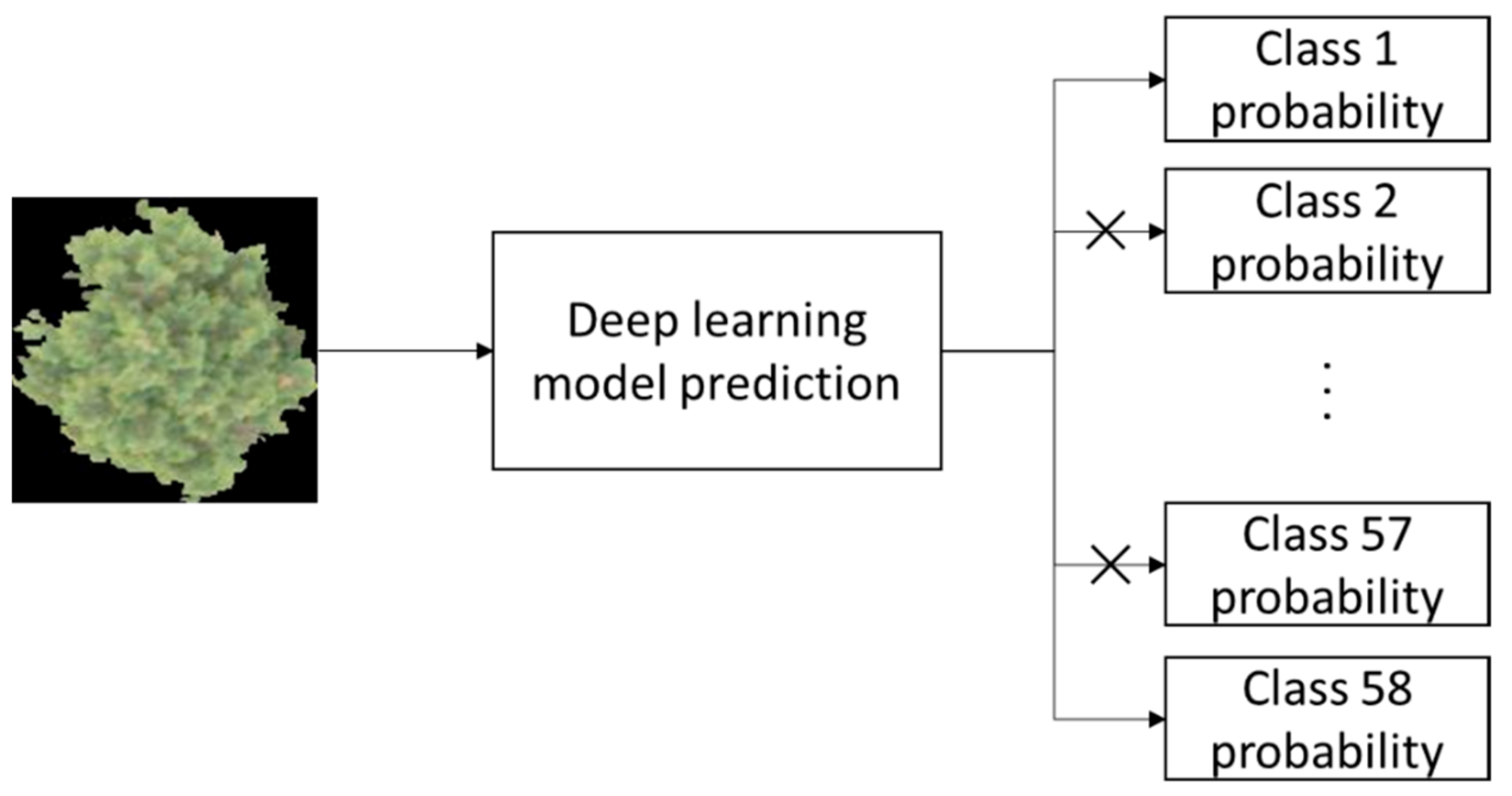
2.5. Deep Learning
2.6. Analysis
2.7. Performance Evaluation
3. Results
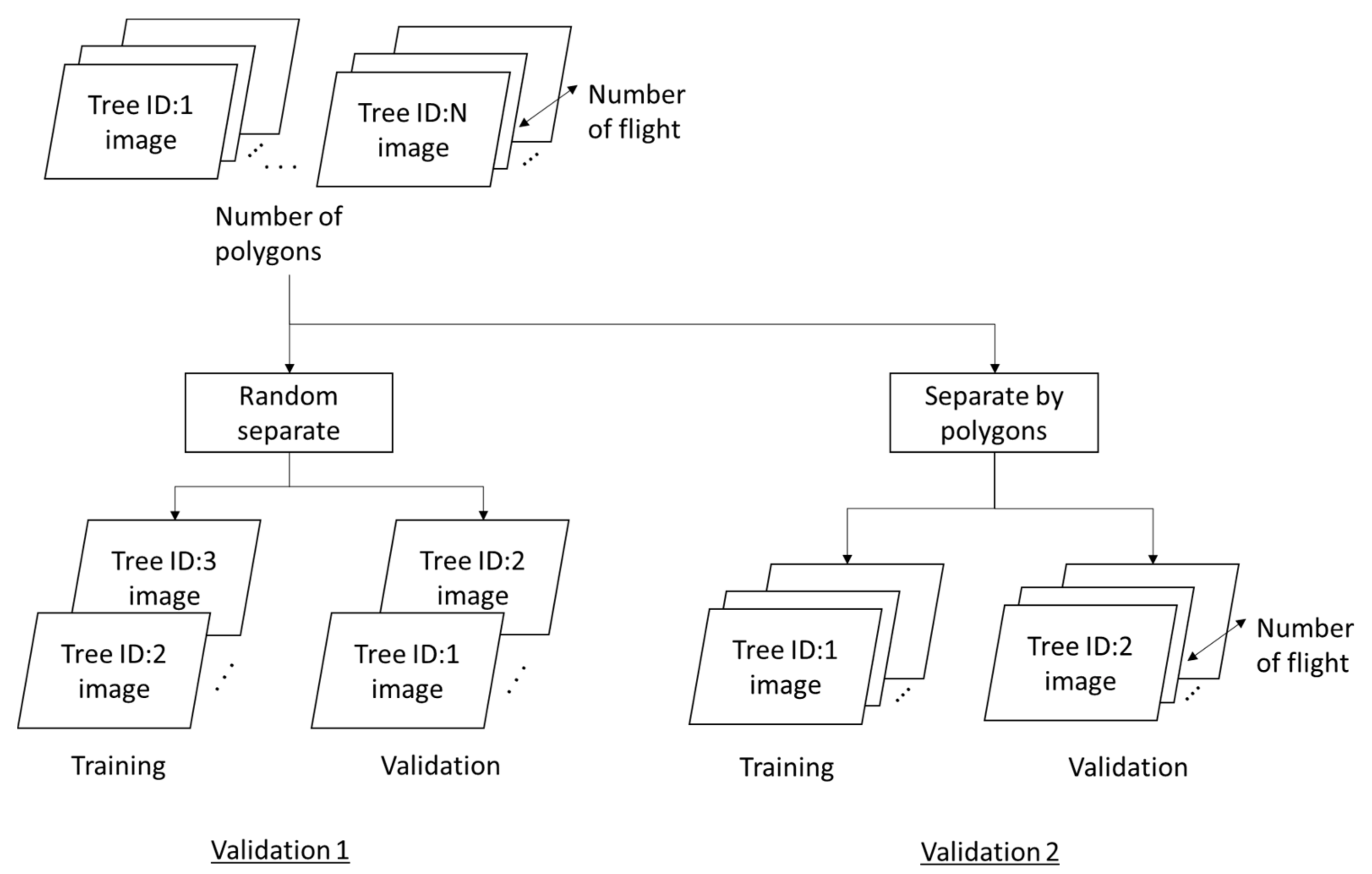
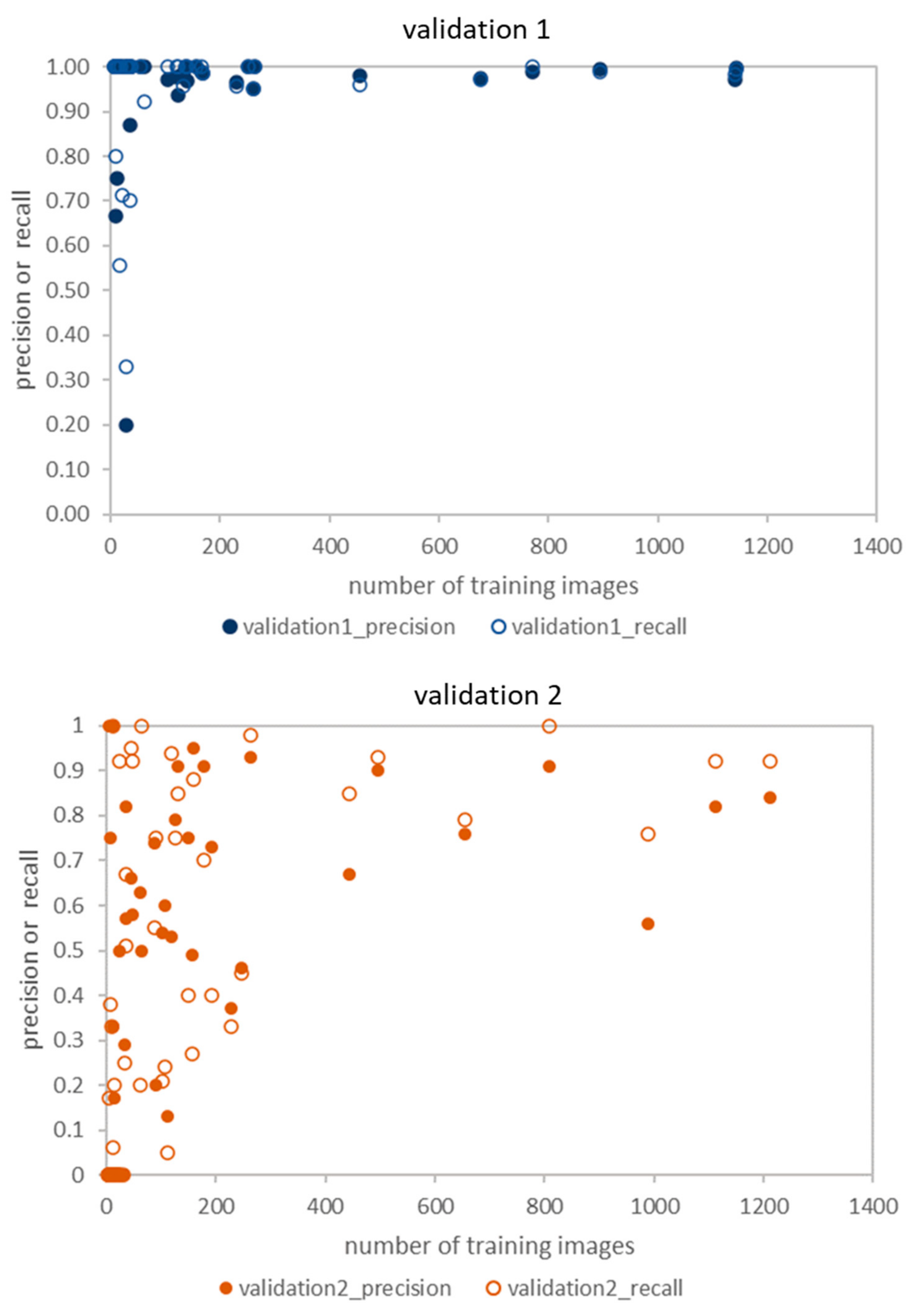
3.1. Validation 1: Performance for Dataset of Same Acquisition Date or Same Individual Trees
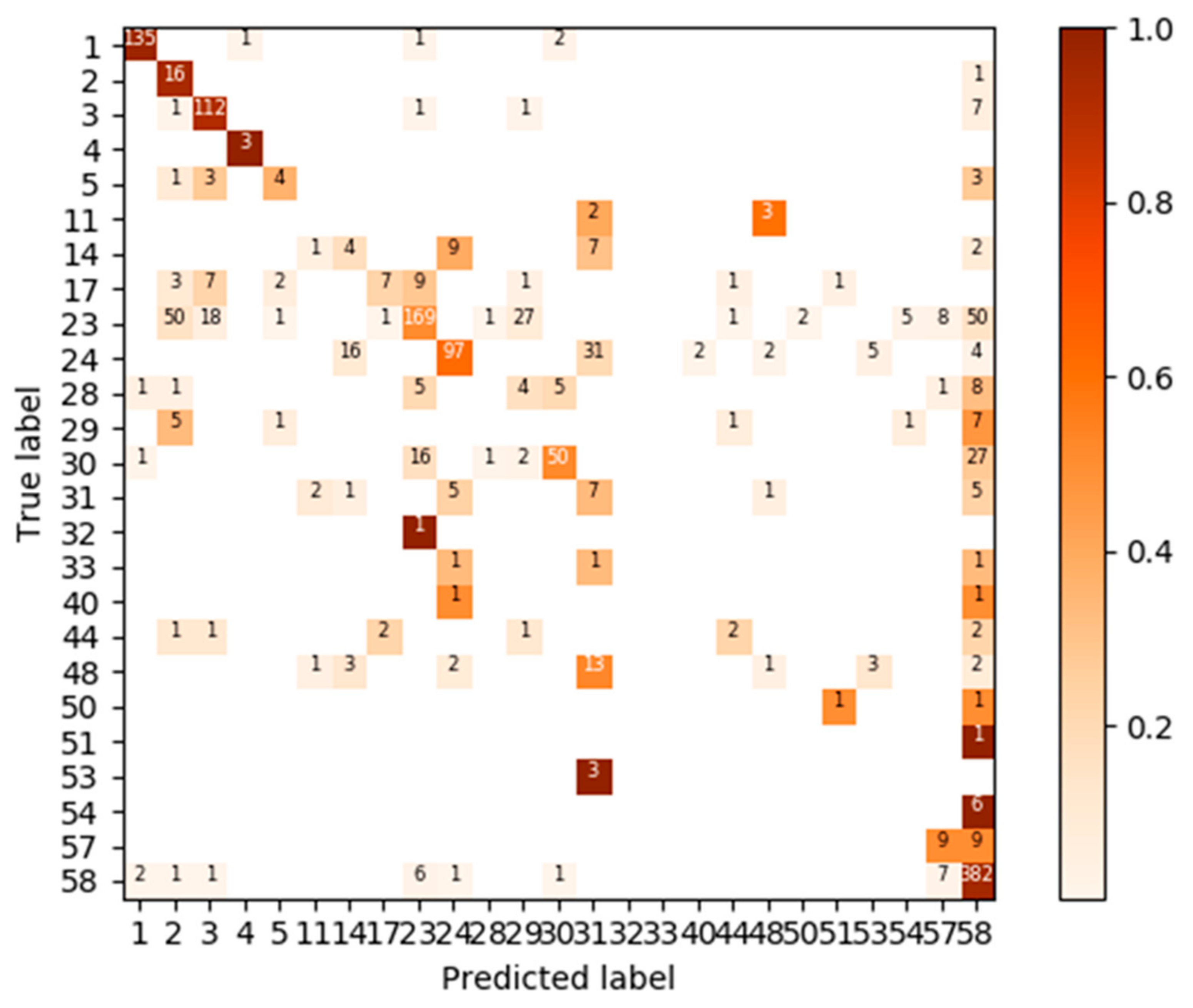
3.2. Validation 2: Performance for Dataset of Same Acquisition Date and Different Individual Trees
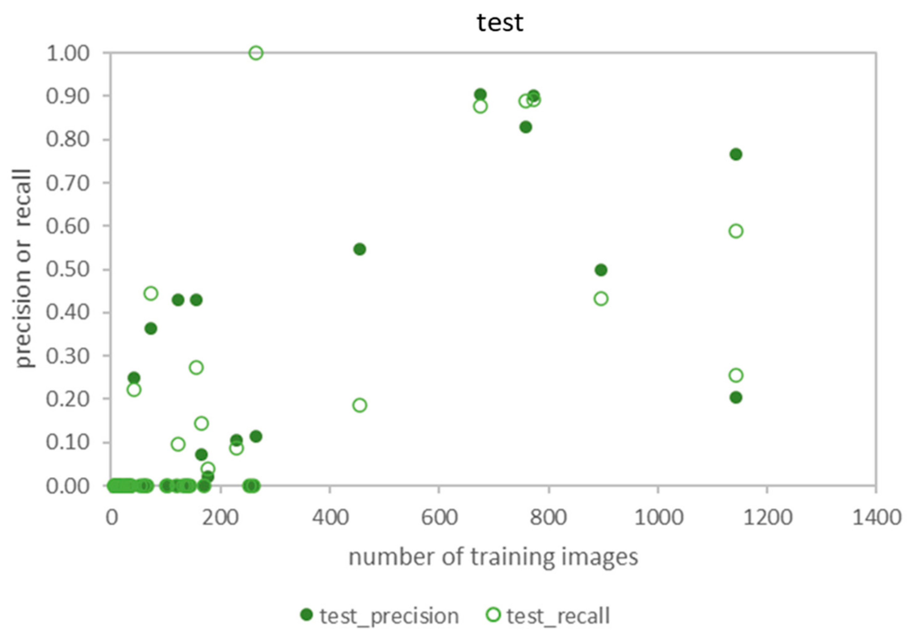
3.3. Test: Performance for Dataset of Different Acquisition Date and Different Site
3.4. Test Using Inventory Tuning
3.5. The Relationship between Accuracy and the Number of Training Images
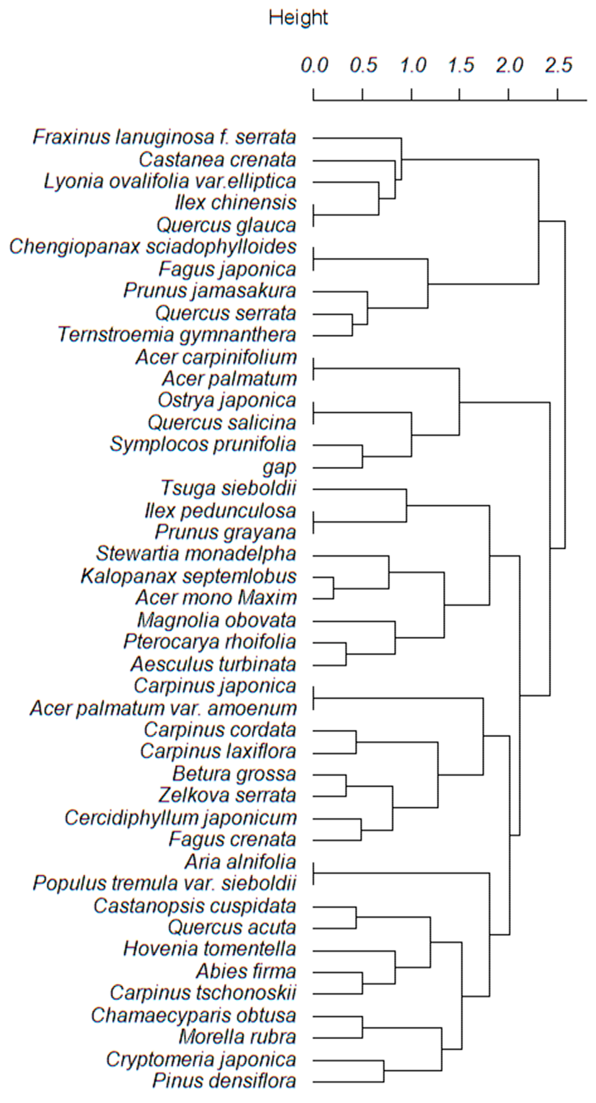
3.6. Similarities in Appearance of Trees Species
4. Discussion
4.1. Classification Performance and Robustness
4.2. Inventory Tuning
4.3. Similarities in Appearance of Trees Species
4.4. Future Study
5. Conclusions
Supplementary Materials
Author Contributions
Funding
Institutional Review Board Statement
Informed Consent Statement
Data Availability Statement
Acknowledgments
Conflicts of Interest
References
- Shang, X.; Chisholm, L.A. Classification of Australian native forest species using hyperspectral remote sensing and machine-learning classification algorithms. IEEE J. Sel. Top. Appl. Earth Obs. Remote Sens. 2014, 7, 2481–2489. [Google Scholar] [CrossRef]
- Boschetti, M.; Boschetti, L.; Oliveri, S.; Casati, L.; Canova, I. Tree species mapping with airborne hyper-spectral MIVIS data: The Ticino Park study case. Int. J. Remote Sens. 2007, 28, 1251–1261. [Google Scholar] [CrossRef]
- Jansson, G.; Angelstam, P. Threshold levels of habitat composition for the presence of the long-tailed tit (Aegithalos caudatus) in a boreal landscape. Landsc. Ecol. 1999, 14, 283–290. [Google Scholar] [CrossRef]
- Forestry Agency. Annual Report on Forest and Forestry in Japan, Fiscal Year 2020; Forestry Agency: Tokyo, Japan, 2020; Available online: https://www.rinya.maff.go.jp/j/kikaku/hakusyo/R2hakusyo/index.html (accessed on 6 February 2022).
- Fassnacht, F.E.; Latifi, H.; Stereńczak, K.; Modzelewska, A.; Lefsky, M.; Waser, L.T.; Straub, C.; Ghosh, A. Review of studies on tree species classification from remotely sensed data. Remote Sens. Environ. 2016, 186, 64–87. [Google Scholar] [CrossRef]
- Dalponte, M.; Bruzzone, L.; Gianelle, D. Tree species classification in the Southern Alps based on the fusion of very high geometrical resolution multispectral/hyperspectral images and LiDAR data. Remote Sens. Environ. 2012, 123, 258–270. [Google Scholar] [CrossRef]
- Shen, X.; Cao, L. Tree-species classification in subtropical forests using airborne hyperspectral and LiDAR data. Remote Sens. 2017, 9, 1180. [Google Scholar] [CrossRef] [Green Version]
- Asner, G.P. Biophysical and biochemical sources of variability in canopy reflectance. Remote Sens. Environ. 1998, 64, 234–253. [Google Scholar] [CrossRef]
- Clark, M.L.; Roberts, D.A. Species-level differences in hyperspectral metrics among tropical rainforest trees as determined by a tree-based classifier. Remote Sens. 2012, 4, 1820–1855. [Google Scholar] [CrossRef] [Green Version]
- Knipling, E.B. Physical and physiological basis for the reflectance of visible and near-infrared radiation from vegetation. Remote Sens. Environ. 1970, 1, 155–159. [Google Scholar] [CrossRef]
- Ustin, S.L.; Gitelson, A.A.; Jacquemoud, S.; Schaepman, M.; Asner, G.P.; Gamon, J.A.; Zarco-Tejada, P. Retrieval of foliar information about plant pigment systems from high resolution spectroscopy. Remote Sens. Environ. 2009, 113, S67–S77. [Google Scholar] [CrossRef] [Green Version]
- Clark, M.L.; Roberts, D.A.; Clark, D.B. Hyperspectral discrimination of tropical rain forest tree species at leaf to crown scales. Remote Sens. Environ. 2005, 96, 375–398. [Google Scholar] [CrossRef]
- Grant, L. Diffuse and specular characteristics of leaf reflectance. Remote Sens. Environ. 1987, 22, 309–322. [Google Scholar] [CrossRef]
- Nakatake, S.; Yamamoto, K.; Yoshida, N.; Yamaguchi, A.; Unom, S. Development of a single tree classification method using airborne LiDAR. J. Jpn. For. Soc. 2018, 100, 149–157. [Google Scholar] [CrossRef] [Green Version]
- Zhang, C.; Qiu, F. Mapping individual tree species in an urban forest using airborne lidar data and hyperspectral imagery. Photogramm. Eng. Remote Sens. 2012, 78, 1079–1087. [Google Scholar] [CrossRef] [Green Version]
- Schreyer, J.; Tigges, J.; Lakes, T.; Churkina, G. Using airborne LiDAR and QuickBird data for modelling urban tree carbon storage and its distribution-a case study of Berlin. Remote Sens. 2014, 6, 10636–10655. [Google Scholar] [CrossRef] [Green Version]
- Rahman, M.T.; Rashed, T. Urban tree damage estimation using airborne laser scanner data and geographic information systems: An example from 2007 Oklahoma ice storm. Urban For. Urban Green. 2015, 14, 562–572. [Google Scholar] [CrossRef]
- Zhang, Z.; Kazakova, A.; Moskal, L.M.; Styers, D.M. Object-based tree species classification in urban ecosystems using LiDAR and hyperspectral data. Forests 2016, 7, 122. [Google Scholar] [CrossRef] [Green Version]
- Ballanti, L.; Blesius, L.; Hines, E.; Kruse, B. Tree species classification using hyperspectral imagery: A comparison of two classifiers. Remote Sens. 2016, 8, 445. [Google Scholar] [CrossRef] [Green Version]
- Cao, L.; Coops, N.C.; Innes, J.L.; Dai, J.; Ruan, H.; She, G. Tree species classification in subtropical forests using small-footprint full-waveform LiDAR data. Int. J. Appl. Earth Obs. Geoinf. 2016, 49, 39–51. [Google Scholar] [CrossRef]
- Dalponte, M.; Bruzzone, L.; Vescovo, L.; Gianelle, D. The role of spectral resolution and classifier complexity in the analysis of hyperspectral images of forest areas. Remote Sens. Environ. 2009, 113, 2345–2355. [Google Scholar] [CrossRef]
- Dalponte, M.; Ørka, H.O.; Gobakken, T.; Gianelle, D.; Næsset, E. Tree species classification in boreal forests with hyperspectral data. IEEE Trans. Geosci. Remote Sens. 2013, 51, 2632–2645. [Google Scholar] [CrossRef]
- Feret, J.B.; Asner, G.P. Tree species discrimination in tropical forests using airborne imaging spectroscopy. IEEE Trans. Geosci. Remote Sens. 2013, 51, 73–84. [Google Scholar] [CrossRef]
- Machala, M.; Zejdová, L. Forest mapping through object-based image analysis of multispectral and LiDAR aerial data. Eur. J. Remote Sens. 2014, 47, 117–131. [Google Scholar] [CrossRef]
- Waser, L.T.; Küchler, M.; Jütte, K.; Stampfer, T. Evaluating the potential of worldview-2 data to classify tree species and different levels of ash mortality. Remote Sens. 2014, 6, 4515–4545. [Google Scholar] [CrossRef] [Green Version]
- Nevalainen, O.; Honkavaara, E.; Tuominen, S.; Viljanen, N.; Hakala, T.; Yu, X.; Hyyppä, J.; Saari, H.; Pölönen, I.; Imai, N.N.; et al. Individual tree detection and classification with UAV-Based photogrammetric point clouds and hyperspectral imaging. Remote Sens. 2017, 9, 185. [Google Scholar] [CrossRef] [Green Version]
- Sothe, C.; Dalponte, M.; de Almeida, C.M.; Schimalski, M.B.; Lima, C.L.; Liesenberg, V.; Miyoshi, G.T.; Tommaselli, A.M.G. Tree species classification in a highly diverse subtropical forest integrating UAV-based photogrammetric point cloud and hyperspectral data. Remote Sens. 2019, 11, 1338. [Google Scholar] [CrossRef] [Green Version]
- Natesan, S.; Armenakis, C.; Vepakomma, U. Resnet-based tree species classification using uav images. Int. Arch. Photogramm. Remote Sens. Spat. Inf. Sci. 2019, XLII, 475–481. [Google Scholar] [CrossRef] [Green Version]
- Onishi, M.; Ise, T. Explainable identification and mapping of trees using UAV RGB image and deep learning. Sci. Rep. 2021, 11, 903. [Google Scholar] [CrossRef]
- Safonova, A.; Tabik, S.; Alcaraz-Segura, D.; Rubtsov, A.; Maglinets, Y.; Herrera, F. Detection of fir trees (Abies sibirica) damaged by the bark beetle in unmanned aerial vehicle images with deep learning. Remote Sens. 2019, 11, 643. [Google Scholar] [CrossRef] [Green Version]
- Ishihara, M.; Ishida, K.; Ida, H.; Itoh, A.; Enoki, T.; Ohkubo, T.; Kaneko, T.; Kaneko, N.; Kuramoto, S.; Sakai, T.; et al. An introduction to forest permanent plot data at Core and Subcore sites of the Forest and Grassland Survey of the Monitoring Sites 1000 Project(News). Jpn. J. Ecol. 2010, 60, 111–123. [Google Scholar]
- Baatz, M.; Schäpe, A. Multiresolution segmentation: An optimization approach for high quality multi-scale image segmentation. In XII Angewandte Geographische Information; Wichmann-Verlag: Heidelberg, Germany, 2000; pp. 12–23. [Google Scholar]
- Paszke, A.; Gross, S.; Chintala, S.; Chanan, G.; Yang, E.; DeVito, Z.; Lin, Z.; Desmaison, A.; Antiga, L.; Lerer, A. Automatic differentiation in PyTorch. In Proceedings of the 31st Conference on Neural Information Processing System, Long Beach, CA, USA, 4–9 December 2017. [Google Scholar] [CrossRef]
- Tan, M.; Le, Q.V. EfficientNet: Rethinking model scaling for convolutional neural networks. In Proceedings of the 36th International Conference on Machine Learning, ICML 2019, Long Beach, CA, USA, 9–15 June 2019; pp. 10691–10700. [Google Scholar]
- Cohen, J. A coeffient of agreement for nominal scales. Educ. Psychol. Meas. 1960, 20, 37–46. [Google Scholar] [CrossRef]
- Ward, J.H. Hierarchical Grouping to Optimize an Objective Function. J. Am. Stat. Assoc. 1963, 58, 236–244. [Google Scholar] [CrossRef]
- Dalponte, M.; Bruzzone, L.; Gianelle, D. Fusion of hyperspectral and LIDAR remote sensing data for classification of complex forest areas. IEEE Trans. Geosci. Remote Sens. 2008, 46, 1416–1427. [Google Scholar] [CrossRef] [Green Version]
- Gewali, U.B.; Monteiro, S.T.; Saber, E. Machine learning based hyperspectral image analysis: A survey. arXiv 2018, arXiv:1802.08701. [Google Scholar]
- Goodwin, N.; Turner, R.; Merton, R. Classifying Eucalyptus forests with high spatial and spectral resolution imagery: An investigation of individual species and vegetation communities. Aust. J. Bot. 2005, 53, 337–345. [Google Scholar] [CrossRef]
- Youngentob, K.N.; Roberts, D.A.; Held, A.A.; Dennison, P.E.; Jia, X.; Lindenmayer, D.B. Mapping two Eucalyptus subgenera using multiple endmember spectral mixture analysis and continuum-removed imaging spectrometry data. Remote Sens. Environ. 2011, 115, 1115–1128. [Google Scholar] [CrossRef]
- Chen, Q.; Baldocchi, D.; Gong, P.; Kelly, M. Isolating individual trees in a savanna woodland using small footprint lidar data. Photogramm. Eng. Remote Sens. 2006, 72, 923–932. [Google Scholar] [CrossRef] [Green Version]
- Jakubowski, M.K.; Li, W.; Guo, Q.; Kelly, M. Delineating individual trees from lidar data: A comparison of vector- and raster-based segmentation approaches. Remote Sens. 2013, 5, 4163–4186. [Google Scholar] [CrossRef] [Green Version]
- Ke, Y.; Quackenbush, L.J. A review of methods for automatic individual tree-crown detection and delineation from passive remote sensing. Int. J. Remote Sens. 2011, 32, 4725–4747. [Google Scholar] [CrossRef]
- Koch, B.; Heyder, U.; Welnacker, H. Detection of individual tree crowns in airborne lidar data. Photogramm. Eng. Remote Sens. 2006, 72, 357–363. [Google Scholar] [CrossRef] [Green Version]
- Solberg, S.; Naesset, E.; Bollandsas, O.M. Single tree segmentation using airborne laser scanner data in a structurally heterogeneous spruce forest. Photogramm. Eng. Remote Sens. 2006, 72, 1369–1378. [Google Scholar] [CrossRef]
- Wulder, M.; Niemann, K.O.; Goodenough, D.G. Local maximum filtering for the extraction of tree locations and basal area from high spatial resolution imagery. Remote Sens. Environ. 2000, 73, 103–114. [Google Scholar] [CrossRef]
- Picos, J.; Bastos, G.; Míguez, D.; Alonso, L.; Armesto, J. Individual tree detection in a eucalyptus plantation using unmanned aerial vehicle (UAV)-LiDAR. Remote Sens. 2020, 12, 885. [Google Scholar] [CrossRef] [Green Version]
- Mohan, M.; Silva, C.A.; Klauberg, C.; Jat, P.; Catts, G.; Cardil, A.; Hudak, A.T.; Dia, M. Individual tree detection from unmanned aerial vehicle (UAV) derived canopy height model in an open canopy mixed conifer forest. Forests 2017, 8, 340. [Google Scholar] [CrossRef] [Green Version]
- Dalponte, M.; Frizzera, L.; Gianelle, D. Individual tree crown delineation and tree species classification with hyperspectral and LiDAR data. PeerJ 2019, 6, e6227. [Google Scholar] [CrossRef]
- Maschler, J.; Atzberger, C.; Immitzer, M. Individual tree crown segmentation and classification of 13 tree species using Airborne hyperspectral data. Remote Sens. 2018, 10, 1218. [Google Scholar] [CrossRef] [Green Version]
- He, K.; Zhang, X.; Ren, S.; Sun, J. Deep residual learning for image recognition. In Proceedings of the 2016 IEEE Conference on Computer Vision and Pattern Recognition (CVPR), Las Vegas, NV, USA, 27–30 June 2016; pp. 770–778. [Google Scholar] [CrossRef] [Green Version]
- Tucker, C.J. Red and photographic infrared linear combinations for monitoring vegetation. Remote Sens. Environ. 1979, 8, 127–150. [Google Scholar] [CrossRef] [Green Version]
- Bendig, J.; Yu, K.; Aasen, H.; Bolten, A.; Bennertz, S.; Broscheit, J.; Gnyp, M.L.; Bareth, G. Combining UAV-based plant height from crop surface models, visible, and near infrared vegetation indices for biomass monitoring in barley. Int. J. Appl. Earth Obs. Geoinf. 2015, 39, 79–87. [Google Scholar] [CrossRef]


| Site Name | Higashiyama | Wakayama | Ashiu |
| Data class | Training | Training | Training |
| Field research area | 2 ha | 1 ha | 4 ha |
| Flight date | 4, 5 July and 14, 15 September 2019 | 15, 17 July and 8 October 2019 | 24–26 July and 18–20 September 2019 |
| dominant species | Castanopsis cuspidate Quercus serrata | Abies firma, Tsuga sieboldii | Fagus crenata Cryptomeria japonica |
| Site Name | Kamigamo | Kasugayama | Daisen |
| Data class | Test | Test | Test |
| Field research area | 1.5 ha | 1 ha | 1 ha |
| Flight date | 10 October 2019 | 24 September 2019 | 1 October 2019 |
| dominant species | Chamaecyparis obtusa Quercus serrata | Castanopsis cuspidate Abies firma | Fagus crenata |
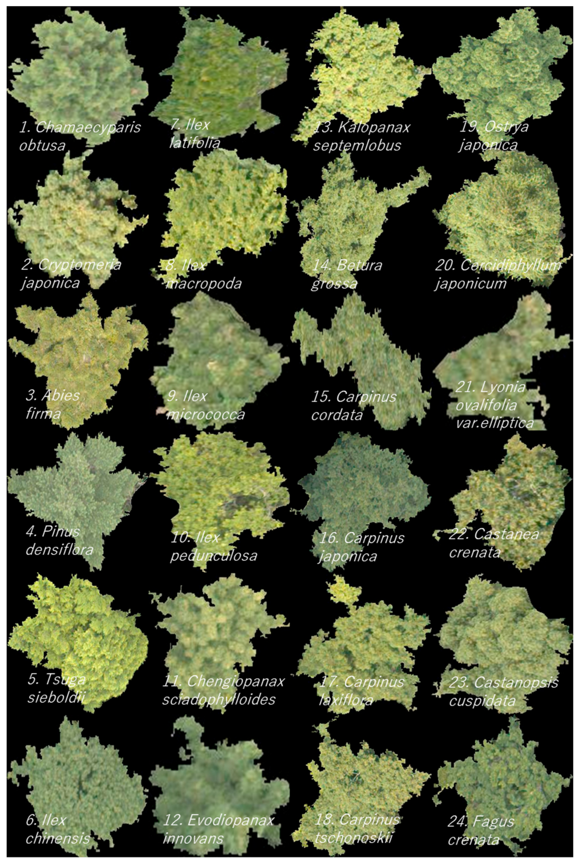
| Class | Species Name | Class | Species Name |
|---|---|---|---|
| 1 | Chamaecyparis obtusa | 30 | Quercus serrata |
| 2 | Cryptomeria japonica | 31 | Pterocarya rhoifolia |
| 3 | Abies firma | 32 | Cinnamomum camphora |
| 4 | Pinus densiflora | 33 | Magnolia obovata |
| 5 | Tsuga sieboldii | 34 | Magnolia salicifolia |
| 6 | Ilex chinensis | 35 | Morella rubra |
| 7 | Ilex latifolia | 36 | Fraxinus lanuginosa f. serrata |
| 8 | Ilex macropoda | 37 | Ternstroemia gymnanthera |
| 9 | Ilex micrococca | 38 | Hovenia dulcis |
| 10 | Ilex pedunculosa | 39 | Hovenia tomentella |
| 11 | Chengiopanax sciadophylloides | 40 | Aria alnifolia |
| 12 | Evodiopanax innovans | 41 | Aria japonica |
| 13 | Kalopanax septemlobus | 42 | Malus tschonoskii |
| 14 | Betura grossa | 43 | Prunus grayana |
| 15 | Carpinus cordata | 44 | Prunus jamasakura |
| 16 | Carpinus japonica | 45 | Meliosma Myriantha |
| 17 | Carpinus laxiflora | 46 | Populus tremula var. sieboldii |
| 18 | Carpinus tschonoskii | 47 | Acer carpinifolium |
| 19 | Ostrya japonica | 48 | Acer mono Maxim |
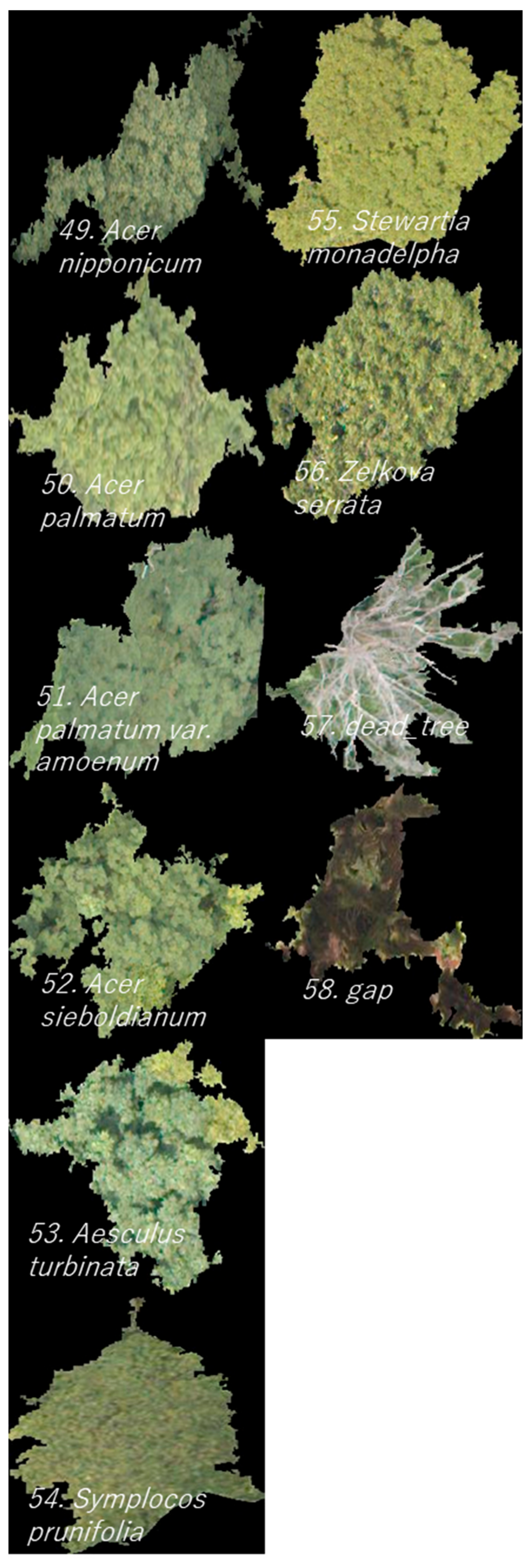
| 20 | Cercidiphyllum japonicum | 49 | Acer nipponicum |
| 21 | Lyonia ovalifolia var.elliptica | 50 | Acer palmatum |
| 22 | Castanea crenata | 51 | Acer palmatum var. amoenum |
| 23 | Castanopsis cuspidata | 52 | Acer sieboldianum |
| 24 | Fagus crenata | 53 | Aesculus turbinata |
| 25 | Fagus japonica | 54 | Symplocos prunifolia |
| 26 | Quercus acuta | 55 | Stewartia monadelpha |
| 27 | Quercus crispula | 56 | Zelkova serrata |
| 28 | Quercus glauca | 57 | dead_tree |
| 29 | Quercus salicina | 58 | Gap |
| Model Prediction | ||||
|---|---|---|---|---|
| Class | A | B | C | |
| Ground truth | A | a | b | c |
| B | d | e | f | |
| C | g | h | We | |
Publisher’s Note: MDPI stays neutral with regard to jurisdictional claims in published maps and institutional affiliations. |
© 2022 by the authors. Licensee MDPI, Basel, Switzerland. This article is an open access article distributed under the terms and conditions of the Creative Commons Attribution (CC BY) license (https://creativecommons.org/licenses/by/4.0/).
Share and Cite
Onishi, M.; Watanabe, S.; Nakashima, T.; Ise, T. Practicality and Robustness of Tree Species Identification Using UAV RGB Image and Deep Learning in Temperate Forest in Japan. Remote Sens. 2022, 14, 1710. https://doi.org/10.3390/rs14071710
Onishi M, Watanabe S, Nakashima T, Ise T. Practicality and Robustness of Tree Species Identification Using UAV RGB Image and Deep Learning in Temperate Forest in Japan. Remote Sensing. 2022; 14(7):1710. https://doi.org/10.3390/rs14071710
Chicago/Turabian StyleOnishi, Masanori, Shuntaro Watanabe, Tadashi Nakashima, and Takeshi Ise. 2022. "Practicality and Robustness of Tree Species Identification Using UAV RGB Image and Deep Learning in Temperate Forest in Japan" Remote Sensing 14, no. 7: 1710. https://doi.org/10.3390/rs14071710